Groups, Lie algebras and gauge theory

8.1 The destination and the route

The expression $SU(3{)}_c\times SU(2{)}_L\times U(1{)}_Y$ becomes useful only when we know what it does. It specifies continuous internal transformations, tells us how fields can transform, and supplies the algebra that organizes their interactions. It does not, by itself, specify every particle, every coupling, or the dynamics of the vacuum. Our aim is to read that expression as a compact set of mathematical instructions.

We will build those instructions in five stages: reversible operations form groups; matrices realize their actions on vectors; differentiating continuous groups gives Lie algebras; representations specify which vectors transform; and comparing transformations at neighboring spacetime points introduces a gauge connection. Its curvature is the gauge field strength.

The prerequisites are matrix multiplication, complex numbers, derivatives, and basic quantum mechanics. Familiarity with fields and special relativity helps in the final third. No previous group theory or differential geometry is assumed. Sections 8.2–8.6 establish the vocabulary; 8.7–8.11 develop the mathematical machinery; 8.12–8.15 build gauge theory; 8.16–8.18 assemble the Standard Model. Worked examples are part of the argument. The exercises in 8.19 are a second pass through its main ideas.

Use the differential geometry Curiosity for a broader account of manifolds, connections, and curvature. The main quantum field theory chapter develops quantization, interactions, anomalies, and the Higgs mechanism beyond this introduction. This is the eighth Curiosity, a separate article from that main physics chapter.

Conventions to keep beside the calculations

Vectors are columns; a product $gh$ acts with $h$ first. The symbol $I$ is an identity matrix; $e$ is a group's identity unless explicitly identified as the electromagnetic coupling. A dagger means conjugate transpose. Summed repeated Lie-algebra indices are understood. Spacetime indices are $\mu ,\nu =0,1,2,3$.

For quantum fields we use natural units $\hslash =c=1$ and Minkowski signature $(+,-,-,-)$. Internal generators $t_a$ are Hermitian, with

$$[t_a,t_b]=i{f}_{ab}{}^c{t}_c,\mathrm{tr}(t_a{t}_b)=\frac{1}{2}{\delta }_{ab}$$

in the defining representation of $SU(N)$. The trace normalization is a choice, not an axiom applying to every representation. Our gauge conventions are

$${\psi }^{\prime }=U\psi ,D_{\mu }={\partial }_{\mu }-ig{A}_{\mu },[D_{\mu },D_{\nu }]=-ig{F}_{\mu \nu }.$$

We will derive their consequences rather than switching signs midway. Hypercharge is defined by $Q=T_3+Y$; a source using $Q=T_3+Y/2$ calls twice our $Y$ its hypercharge. These conventions must travel together when comparing equations.

8.2 What is a group?

A group is a set $G$ together with a binary operation: a rule assigning an element $gh$ of $G$ to each pair $g,h$ in $G$. Four requirements capture what reversible composition needs.

1. Closure: composing two allowed operations gives another allowed operation.
2. Associativity: $(gh)k=g(hk)$. Parentheses may move without changing the answer; the order may not.
3. Identity: there is an element $e$ with $eg=ge=g$.
4. Inverse: each $g$ has an element $g^{-1}$ satisfying $g^{-1}g=g{g}^{-1}=e$.

The operation need not be multiplication of numbers. For integers under addition, the identity is $0$, and the inverse of $n$ is $-n$. Thus $(\mathbb{Z},+)$ is a group. Nonnegative integers under addition fail because a positive integer has no additive inverse within the set. Nonzero real numbers under multiplication form a group; all real numbers under multiplication do not, because $0$ has no multiplicative inverse.

A group is abelian when $gh=hg$ for every pair. Addition of integers is abelian. Compositions of spatial rotations generally are not. Noncommutativity means that the intermediate operation changes the setting in which the next operation acts; it does not mean that composition is inconsistent.

Worked example 1: a clock with five positions

Let ${\mathbb{Z}}_5$ consist of the residue classes $0,1,2,3,4$, with addition modulo $5$. Then

$$3+4=2(\mathrm{mod}5),-3=2(\mathrm{mod}5).$$

The element $1$ generates the whole group: repeated addition visits all five positions. Equivalently, write the cyclic group as $C_5=\{e,r,r^2,r^3,r^4\}$ with $r^5=e$. Its order, meaning its number of elements, is five. In a continuous group, the number of real parameters is instead called its dimension; these are different concepts.

Associativity lets us solve equations without assuming commutativity. From $gx=h$, multiply on the left by $g^{-1}$ to obtain $x=g^{-1}h$. Multiplication on the wrong side would generally fail. Similarly,

$$(gh{)}^{-1}=h^{-1}{g}^{-1},$$

because undoing a sequence requires undoing its last step first. This simple identity will reappear in matrix algebra and gauge transformations.

A subgroup is a subset that is itself a group under the same operation. For example, the multiples of five form a subgroup of $(\mathbb{Z},+)$. A homomorphism is a map preserving multiplication, $\rho (gh)=\rho (g)\rho (h)$. It preserves identity and inverses automatically. When such a map is bijective, it is an isomorphism: two presentations have the same abstract group structure.

Checkpoint. Associativity does not assert $gh=hg$. It only says that executing three operations does not depend on where we place the bookkeeping parentheses.

8.3 Symmetries act: the triangle as a laboratory

An abstract group need not come with a particular object to transform. A group action supplies that object: for a set $X$, it assigns $g\cdot x$ so that $e\cdot x=x$ and $(gh)\cdot x=g\cdot (h\cdot x)$. The same group can act on positions, functions, quantum states, or internal field components.

Label the vertices of an equilateral triangle $1,2,3$. Let $r=(123)$ cycle them, and let $s=(23)$ fix vertex $1$ while exchanging vertices $2$ and $3$. In cycle notation, $(123)$ means $1\mapsto 2$, $2\mapsto 3$, $3\mapsto 1$. The six triangle symmetries form the dihedral group $D_3$, isomorphic to the permutation group $S_3$:

$$D_3=\{e,r,r^2,s,sr,s{r}^2\},r^3=e,s^2=e,srs=r^{-1}.$$

The first two relations express three rotations and two reflections returning to the start. The third says that reflecting reverses the sense of rotation.

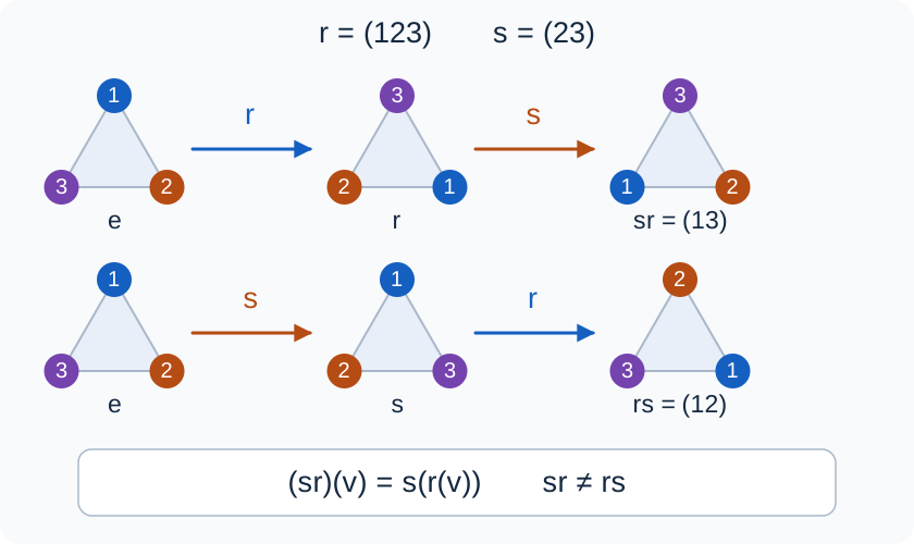
The colored vertices keep track of the action. Both sequences use the same two operations, but $sr$ and $rs$ exchange different vertex pairs.

Worked example 2: calculate the failure to commute

For $sr$, follow vertex $1$: $r$ sends it to $2$, then $s$ sends $2$ to $3$. Vertex $3$ goes first to $1$, then stays there. Vertex $2$ returns to itself. Therefore $sr=(13)$. Conversely, $rs$ sends $1$ to $2$, $2$ to $1$, and fixes $3$, so $rs=(12)$. Hence $sr\ne rs$.

The orbit of a point is the set of places the group can send it. The orbit of vertex $1$ contains all three vertices. Its stabilizer consists of operations leaving it fixed: $\{e,s\}$. The finite orbit–stabilizer relation is visible here:

$$|D_3|=|\mathrm{Orb}(1)||\mathrm{Stab}(1)|=3\times 2.$$

The kernel of an action contains elements acting trivially on every point. This triangle action has only the identity in its kernel and is called faithful. An unfaithful action can hide part of the group. Later, ordinary three-dimensional vectors will be unable to distinguish two different elements of $SU(2)$.

There is also a useful distinction between an active transformation and a passive change of description. Actively rotate a vector by a matrix $R$, keeping the axes fixed: $v^{\prime }=Rv$. Passively rotate the axes while leaving the geometric vector fixed: its components transform by $R^{-1}$. Either convention works. Confusing the two produces apparent sign disagreements, especially for rotations and gauge frames.

Checkpoint. A symmetry is specified by both a group element and what it acts on. A group element invisible in one action can be visible in another.

8.4 Matrices, complex numbers, and preserved quantities

A linear transformation sends sums to sums and scalar multiples to scalar multiples. Choosing a basis represents it by a matrix. Composition becomes matrix multiplication; an invertible matrix describes a reversible linear transformation. The invertible $n\times n$ matrices over a field $\mathbb{F}$ form $GL(n,\mathbb{F})$, the general linear group.

Why select a smaller group? Usually a physical quantity must be preserved. For real vectors with squared Euclidean length $v^{T}v$, a matrix $R$ preserves every length precisely when

$$(Rv{)}^T(Rv)=v^T{R}^{T}Rv=v^{T}v,R^{T}R=I.$$

These are orthogonal matrices, forming $O(n)$. Their determinants obey $(\det R{)}^2=1$, so $\det R=\pm 1$. Requiring $+1$ selects $SO(n)$, the special orthogonal group. Reflections have determinant $-1$ and are excluded; rotations belong to $SO(n)$.

For complex vectors, the nonnegative squared norm is $z^{†}z$, not $z^{T}z$. A matrix preserving it obeys $U^{†}U=I$ and is unitary. Such matrices form $U(n)$; adding $\det U=1$ gives $SU(n)$. Here “special” means determinant one, and “unitary” means preservation of a Hermitian inner product. Neither word says that the matrix entries are real.

Worked example 3: a complex phase is a real rotation

Write $z=x+iy$. Multiplying by $e^{i\theta }=\cos \theta +i\sin \theta$ gives

$$e^{i\theta }z=(x\cos \theta -y\sin \theta )+i(x\sin \theta +y\cos \theta ).$$

Thus one complex component transforms exactly like two real components:

$$\left(\begin{array}{c}{x}^{\prime }\\ y^{\prime }\end{array}\right)=\left(\begin{array}{cc}\cos \theta & -\sin \theta \\ \sin \theta & \cos \theta \end{array}\right)\left(\begin{array}{c}x\\ y\end{array}\right).$$

The modulus $|z|$ is unchanged. The set of phases $e^{i\theta }$ forms $U(1)$, and this correspondence is a group isomorphism $U(1)\cong SO(2)$. It does not identify every physical use of the groups: a phase acting on an electron field is an internal transformation, whereas a rotation of a laboratory plane acts on spatial positions.

Quantum mechanics makes complex inner products particularly important. Unitary transformations preserve transition probabilities because $⟨U\varphi ,U\psi ⟩=⟨\varphi ,\psi ⟩$. A Hermitian matrix satisfies $H^{†}=H$ and can represent an observable. It is generally not itself a group transformation. Instead, $e^{i\alpha H}$ is unitary for real $\alpha$, which is the bridge between observables or generators and finite transformations.

For example, $\mathrm{diag}(1,-1)$ is both Hermitian and unitary, but $\mathrm{diag}(2,3)$ is Hermitian without being unitary. Hermitian and unitary are different conditions with different roles.

8.5 Continuous rotations and the phase circle

The matrix from the previous section will be denoted $R(\theta )$. Direct multiplication, using the angle-addition formulas, gives

$$R(\alpha )R(\beta )=R(\alpha +\beta ),R(\theta {)}^{-1}=R(-\theta ).$$

One parameter labels planar rotations, but the parameter is periodic: $\theta$ and $\theta +2\pi$ describe the same element. The group is a circle rather than an infinite line. Locally, a small interval of angles is enough; globally, those intervals must fit around the circle.

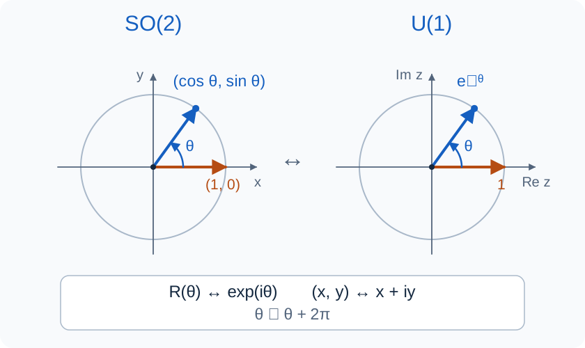
The real matrix $R(\theta )$ and the complex number $e^{i\theta }$ realize the same one-parameter composition law.

Worked example 4: the infinitesimal rotation

For a small angle $ϵ$,

$$R(ϵ)=I+ϵJ+O({ϵ}^2),J=\left(\begin{array}{cc}0& -1\\ 1& 0\end{array}\right),J^2=-I.$$

Separate the even and odd powers in the exponential series:

$$e^{\theta J}=I\left(1-\frac{{\theta }^2}{2!}+\cdots \right)+J\left(\theta -\frac{{\theta }^3}{3!}+\cdots \right)=I\cos \theta +J\sin \theta =R(\theta ).$$

This is already Lie theory: one infinitesimal direction $J$ generates an entire continuous family.

Three-dimensional rotations have three independent infinitesimal directions. They do not commute. To see it without abstract notation, begin with $v=(1,0,0{)}^T$. A positive right-handed rotation $R_y(\pi /2)$ sends $v$ to $(0,0,-1{)}^T$, and then $R_z(\pi /2)$ leaves that vector fixed. Reversing the order first gives $(0,1,0{)}^T$, which $R_y(\pi /2)$ leaves fixed. Hence

$$R_z(\pi /2)R_y(\pi /2)v\ne R_y(\pi /2)R_z(\pi /2)v.$$

An angle and an axis can describe a three-dimensional rotation, but this does not mean four independent parameters: a unit axis has two parameters and the angle adds one. At zero angle all axes describe the same identity, so this parametrization also warns us that coordinates on a group may have redundancies or singularities.

Checkpoint. The periodic angle of $U(1)$ and the real infinitesimal parameter describing motion near its identity are not the same global space.

8.6 Lie groups: a group that is also a manifold

A Lie group is a smooth manifold equipped with group multiplication and inversion that are smooth maps. A manifold is a space locally describable by a fixed number of real coordinates, even when no single coordinate system covers the whole space. Smoothness makes differentiation meaningful.

There are therefore two independent structures to remember: the group law tells us how transformations compose, while the manifold tells us how transformations vary continuously. The circle $U(1)$ has both. The additive line $(\mathbb{R},+)$ has both too, but is globally different from a circle.

For a matrix group we can count nearby independent parameters by expanding its defining constraints. This will lead to the tangent space, but first it gives a practical dimension count.

Worked example 5: count the generators before choosing them

Let $U=I+iϵH+O({ϵ}^2)$. Then

$$U^{†}U=I+iϵ(H-H^{†})+O({ϵ}^2),$$

so unitarity requires $H=H^{†}$. An $n\times n$ Hermitian matrix has $n$ real diagonal entries and $n(n-1)/2$ independent complex off-diagonal entries. Its number of real parameters is

$$n+2\frac{n(n-1)}{2}=n^2.$$

The determinant-one condition imposes $\mathrm{tr}H=0$, removing one real parameter. Thus $\dim U(n)=n^2$ and $\dim SU(n)=n^2-1$. Similarly, expanding $R=I+ϵX$ in $R^{T}R=I$ gives $X^T=-X$, with $n(n-1)/2$ independent entries.

Group	Defining matrices	Real group dimension	Dimension of the displayed vector space
$U(1)$	one complex phase	$1$	$1$ complex
$SO(2)$	real orthogonal $2\times 2$, determinant $1$	$1$	$2$ real
$SO(3)$	real orthogonal $3\times 3$, determinant $1$	$3$	$3$ real
$SU(2)$	unitary $2\times 2$, determinant $1$	$3$	$2$ complex
$SU(3)$	unitary $3\times 3$, determinant $1$	$8$	$3$ complex

The last two columns answer different questions. The dimension of $SU(3)$ counts eight independent transformation parameters. Its defining representation acts on a three-component complex vector. Neither number counts generations of quarks.

The rank is another number: for these compact groups, it counts independent commuting generators in a maximal torus. $SU(2)$ has rank one; $SU(3)$ has rank two. Rank is neither group dimension nor representation dimension.

For a precise mathematical treatment of manifolds, smooth group operations, and classical matrix groups, see Etingof's MIT Lie groups notes, Lectures 1–5. The calculations here need only their matrix versions.

8.7 Tangent vectors, generators, and the exponential map

Choose a differentiable curve $g(t)$ in a matrix group with $g(0)=I$. Its initial velocity $X=g^{\prime }(0)$ is a tangent vector at the identity. All such velocities form a real vector space $\mathfrak{g}=T_{e}G$, the underlying vector space of the Lie algebra.

For $U(n)$, differentiating $g(t{)}^{†}g(t)=I$ at $t=0$ gives $X^{†}=-X$. Mathematicians therefore realize $\mathfrak{u}(n)$ as anti-Hermitian matrices, and $\mathfrak{su}(n)$ as traceless anti-Hermitian matrices. Physicists commonly write

$$X=i{\alpha }^a{t}_a,t_a^{†}=t_a,$$

with real coefficients ${\alpha }^a$. The Hermitian $t_a$ are a convenient generator basis; the factor $i$ converts them into actual tangent matrices. Keeping this distinction avoids the false statement that the ordinary commutator of two Hermitian matrices is Hermitian.

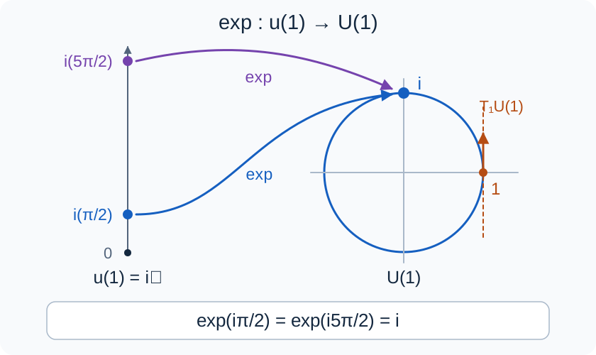
The tangent space records local directions. Exponentiating moves along the group; different tangent-space points can lead to the same group element.

The matrix exponential

$$\exp X=I+X+\frac{X^2}{2!}+\cdots$$

converts an infinitesimal generator into a finite transformation. The curve $g(t)=e^{tX}$ solves $g^{\prime }(t)=Xg(t)$ with $g(0)=I$, and satisfies $g(t+s)=g(t)g(s)$. Such a curve is a one-parameter subgroup.

Worked example 6: why the exponential stays in $SU(n)$

For Hermitian traceless $H$,

$$(e^{iH}{)}^{†}{e}^{iH}=e^{-iH}{e}^{iH}=I,\det (e^{iH})=e^{i\mathrm{tr}H}=1.$$

Thus $e^{iH}$ is special unitary. Conversely, a special unitary matrix can be diagonalized by a unitary change of basis. Its eigenvalues are phases whose angles sum to an integer multiple of $2\pi$; changing one angle by that multiple produces a traceless Hermitian logarithm. Hence every element of $SU(n)$ is an exponential, although the logarithm is not unique.

That final statement is special to this setting. For an arbitrary Lie group, the exponential gives a local coordinate map near the identity, but it need not cover the entire group. Even where it is onto, it is generally not one-to-one. For $U(1)$, $e^{i(\theta +2\pi k)}=e^{i\theta }$ demonstrates the ambiguity directly.

Translation by group multiplication moves tangent vectors at the identity to tangent vectors elsewhere. This is why one tangent space contains enough information to reconstruct local multiplication throughout the identity component. It still does not encode all global identifications or disconnected components. A Lie algebra supplies local structure, not a complete global passport for a group.

8.8 The Lie bracket measures the order of infinitesimal operations

The tangent vector space becomes a Lie algebra when supplied with a bracket. For matrix groups it is the commutator,

$$[X,Y]=XY-YX.$$

It is bilinear, antisymmetric, and satisfies the Jacobi identity,

$$[X,[Y,Z]]+[Y,[Z,X]]+[Z,[X,Y]]=0.$$

These properties are enough to define a Lie algebra abstractly, even without matrices. The bracket must also remain in the algebra. For anti-Hermitian matrices, $[X,Y{]}^{†}=-[X,Y]$; for traceless matrices, $\mathrm{tr}[X,Y]=0$. The matrix constraints are therefore preserved.

Worked example 7: go around a small commutator loop

Expand each exponential to second order and multiply:

$$e^{ϵX}{e}^{ϵY}{e}^{-ϵX}{e}^{-ϵY}=I+{ϵ}^2[X,Y]+O({ϵ}^3).$$

All first-order displacements cancel. What remains measures the mismatch caused by exchanging the order of two infinitesimal transformations. An abelian group gives a zero bracket. A nonzero bracket is the local residue of noncommutativity.

In a Hermitian generator basis, write $[t_a,t_b]=i{f}_{ab}{}^c{t}_c$. The numbers $f_{ab}{}^c$ are structure constants in that basis. They depend on the basis and normalization, while the Lie algebra does not. For compact $SU(N)$ with our trace convention, we can use ${\delta }_{ab}$ to identify upper and lower algebra indices and write $f^{abc}$ as a totally antisymmetric tensor.

The Baker–Campbell–Hausdorff formula organizes the same issue for finite transformations close enough to the identity for the logarithm expansion:

$$\log (e^X{e}^Y)=X+Y+\frac{1}{2}[X,Y]+\frac{1}{12}([X,[X,Y]]+[Y,[Y,X]])+\cdots .$$

Thus $e^X{e}^Y=e^{X+Y}$ is valid when $X$ and $Y$ commute, but is not a general matrix identity. The nested brackets specify the corrections. The formula is a local expansion; it should not be used to claim a globally unique logarithm. Etingof, Lecture 7 gives the precise Lie-theoretic statement.

Checkpoint. “Linearizing the group” does not mean discarding every nonlinear effect. The Lie algebra is a vector space equipped with a bracket that remembers the first nontrivial ordering information.

8.9 Pauli matrices, $SU(2)$, and the double cover of rotations

The Pauli matrices give a concrete Hermitian basis:

$${\sigma }_1=\left(\begin{array}{cc}0& 1\\ 1& 0\end{array}\right),{\sigma }_2=\left(\begin{array}{cc}0& -i\\ i& 0\end{array}\right),{\sigma }_3=\left(\begin{array}{cc}1& 0\\ 0& -1\end{array}\right).$$

Set $t_a={\sigma }_a/2$. Their multiplication law is

$${\sigma }_a{\sigma }_b={\delta }_{ab}I+i{ϵ}_{abc}{\sigma }_c,[t_a,t_b]=i{ϵ}_{abc}{t}_c,\mathrm{tr}(t_a{t}_b)=\frac{1}{2}{\delta }_{ab}.$$

For example, ${\sigma }_1{\sigma }_2=i{\sigma }_3$ while ${\sigma }_2{\sigma }_1=-i{\sigma }_3$, so $[t_1,t_2]=i{t}_3$. Here ${ϵ}_{123}=+1$.

Every $SU(2)$ matrix can be written as $U=a_{0}I+i\mathbf{a}\cdot \mathbf{\sigma }$, with real coefficients satisfying $a_0^2+|\mathbf{a}{|}^2=1$. As a manifold, $SU(2)$ is therefore a three-sphere $S^3$, not the ordinary two-sphere of directions in space.

Worked example 8: a spinor rotation and a vector rotation

To describe an active spatial rotation by angle $\theta$ about unit axis $\mathbf{n}$, use

$$U(\mathbf{n},\theta )=e^{-i\theta \mathbf{n}\cdot \mathbf{\sigma }/2}=I\cos \frac{\theta }{2}-i\mathbf{n}\cdot \mathbf{\sigma }\sin \frac{\theta }{2}.$$

The minus sign is the usual active quantum rotation convention; it corresponds to choosing negative parameters in the general exponential $e^{i{\alpha }^a{t}_a}$. It does not change the Lie algebra or the gauge convention.

Associate a real vector $\mathbf{v}$ with the traceless Hermitian matrix $V=\mathbf{v}\cdot \mathbf{\sigma }$. The transformation $V^{\prime }=UV{U}^{†}$ preserves Hermiticity, trace, and $\det V=-|\mathbf{v}{|}^2$, so it defines an orthogonal transformation of $\mathbf{v}$. Its determinant is $+1$: the action varies continuously, $SU(2)$ is connected, and the identity acts with determinant $+1$. It is therefore a rotation. For the $z$ axis,

$$U{\sigma }_1{U}^{†}=\cos \theta {\sigma }_1+\sin \theta {\sigma }_2,$$

which sends the $x$ direction toward the $y$ direction as expected.

Both $U$ and $-U$ give the same $V^{\prime }$. The map $SU(2)\to SO(3)$ is onto, with kernel $\{I,-I\}$:

$$SO(3)\cong SU(2)/{\mathbb{Z}}_2.$$

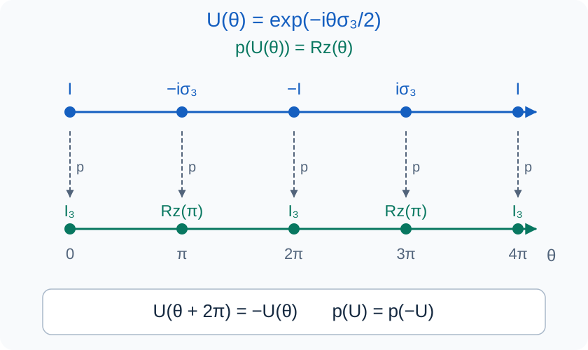
Each spatial rotation has two lifts in $SU(2)$. The diagram follows a single rotation-axis path and does not depict the entire three-sphere.

A two-component spinor transforms by ${\chi }^{\prime }=U\chi$. At $\theta =2\pi$, $U=-I$ and ${\chi }^{\prime }=-\chi$; at $4\pi$, $U=I$. An isolated state and its negative give the same probabilities, but a relative sign between two coherently compared paths can affect interference. The double cover is therefore more than a drawing trick, while it does not mean that a classical arrow requires $4\pi$ to return.

$SU(2)$ and $SO(3)$ have isomorphic Lie algebras but different global representation possibilities. Half-integer-spin representations are representations of $SU(2)$ and do not descend to ordinary single-valued representations of $SO(3)$. See Etingof, Example 2.13 and the covering discussion.

8.10 Representations: the same group, different kinds of objects

A representation on a vector space $V$ is a homomorphism $\rho :G\to GL(V)$. Its defining rule,

$$\rho (gh)=\rho (g)\rho (h),$$

ensures that the matrices respect the abstract composition law. The dimension of the representation is $\dim V$. Differentiating a smooth representation gives generator matrices $T_a$ defined by $d\rho (i{t}_a)=i{T}_a$, so the differential acts on the actual anti-Hermitian tangent matrix. These satisfy the same commutation relations, $[T_a,T_b]=i{f}_{ab}{}^c{T}_c$.

The defining, often called fundamental, representation of $SU(n)$ acts on ${\mathbb{C}}^n$ using its defining matrices. In wider mathematical terminology a simple group can have several fundamental representations; here “the fundamental of $SU(n)$” means this defining $n$-dimensional one. The trivial representation, or singlet, sends every element to $1$.

A representation is irreducible if it has no nonzero proper invariant subspace. “Fundamental” and “irreducible” are not synonyms: many irreducible representations are not the defining one. For compact groups, finite-dimensional unitary representations decompose into direct sums of irreducibles.

A direct sum acts independently on two spaces:

$$({\rho }_1\oplus {\rho }_2)(g)=\left(\begin{array}{cc}{\rho }_1(g)& 0\\ 0& {\rho }_2(g)\end{array}\right),\dim (V\oplus W)=\dim V+\dim W.$$

A tensor product acts on paired components:

$$({\rho }_1\otimes {\rho }_2)(g)(v\otimes w)={\rho }_1(g)v\otimes {\rho }_2(g)w,\dim (V\otimes W)=\dim V\dim W.$$

Differentiating gives total generators $T_a^{\mathrm{total}}=T_a^{(1)}\otimes I+I\otimes T_a^{(2)}$. This is the origin of angular-momentum addition.

Worked example 9: two doublets contain a triplet and a singlet

Take two $SU(2)$ doublets with basis $|\uparrow ⟩,|\downarrow ⟩$. Their four-dimensional tensor product splits into the symmetric states

$$|\uparrow \uparrow ⟩,\frac{|\uparrow \downarrow ⟩+|\downarrow \uparrow ⟩}{\sqrt{2}},|\downarrow \downarrow ⟩$$

and the antisymmetric state

$$|s⟩=\frac{|\uparrow \downarrow ⟩-|\downarrow \uparrow ⟩}{\sqrt{2}}.$$

The total $T_3$ has eigenvalues $1,0,-1$ on the symmetric states. All three total generators annihilate $|s⟩$. Thus $2\otimes 2=3\oplus 1$, or $\frac{1}{2}\otimes \frac{1}{2}=1\oplus 0$ in spin notation. The dimensions check: $2\times 2=3+1$.

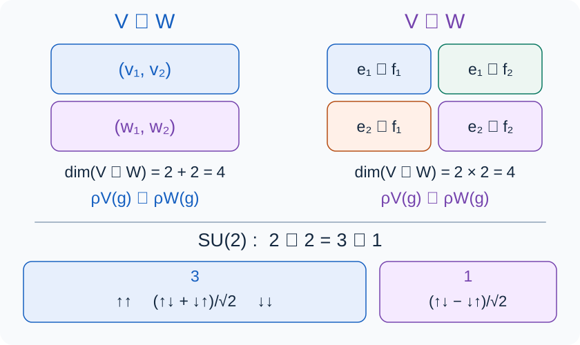
Representations tell us which mathematical objects transform. Combining objects by a tensor product can reveal invariant pieces.

The adjoint representation acts on the Lie algebra itself by conjugation: $X\mapsto gX{g}^{-1}$. Its dimension equals the group dimension. Thus $SU(2)$ has a two-dimensional defining representation and a three-dimensional adjoint; $SU(3)$ has a three-dimensional defining representation and an eight-dimensional adjoint. Gauge curvature transforms in the adjoint. A gauge connection has an additional derivative term, so its full local transformation is not merely an adjoint action.

For $U(1)$, continuous single-valued irreducible unitary representations are ${\rho }_n(e^{i\theta })=e^{in\theta }$ with integer $n$. Periodicity enforces $e^{2\pi in}=1$. Physical charge conventions may rescale these integers together with the coupling; we will explain explicitly how Standard Model fractional hypercharges fit this statement.

8.11 $SU(3)$: three components, eight generators

An $SU(3)$ fundamental vector has three complex components,

$$q=\left(\begin{array}{c}{q}_r\\ q_g\\ q_b\end{array}\right),q^{\prime }=Uq.$$

The color labels red, green, and blue name an internal basis; they are unrelated to optical color or spatial directions. Changing that basis mixes the components while preserving $q^{†}q$. A quark of a fixed flavor is a color triplet. Up, down, and strange are flavor labels and should not be mistaken for the three components of this color representation.

A general traceless Hermitian $3\times 3$ matrix has the form

$$H=\left(\begin{array}{ccc}a& z_1& z_2\\ z_1^{\ast }& b& z_3\\ z_2^{\ast }& z_3^{\ast }& -a-b\end{array}\right).$$

The two real numbers $a,b$ and three complex numbers $z_1,z_2,z_3$ give eight real parameters. This makes the eight generators concrete without requiring us to memorize all eight Gell-Mann matrices.

The conventional basis is $t_a={\lambda }_a/2$. Two diagonal generators are

$$t_3=\frac{1}{2}\left(\begin{array}{ccc}1& 0& 0\\ 0& -1& 0\\ 0& 0& 0\end{array}\right),t_8=\frac{1}{2\sqrt{3}}\left(\begin{array}{ccc}1& 0& 0\\ 0& 1& 0\\ 0& 0& -2\end{array}\right).$$

They commute, giving a rank-two Cartan subalgebra. The other six mix pairs of color components. The upper-left $2\times 2$ Pauli block, completed with a zero third row and column, supplies an $\mathfrak{su}(2)$ subalgebra: $[t_1,t_2]=i{t}_3$. A subgroup inside $SU(3)$ need not be the particular weak $SU(2{)}_L$ of the Standard Model; there those are independent factors acting on different indices.

Worked example 10: a color singlet and a color octet

An antiquark transforms in the complex-conjugate representation $\overline{3}$, using matrices $U^{\ast }$. A quark–antiquark tensor can be arranged as a matrix $M$ transforming by $M\mapsto UM{U}^{†}$. Split it into

$$M=\frac{\mathrm{tr}M}{3}I+\left(M-\frac{\mathrm{tr}M}{3}I\right).$$

The trace part is unchanged by conjugation. The traceless part has eight complex components and transforms in the complexified adjoint representation. Therefore

$$3\otimes \overline{3}=1\oplus 8.$$

The adjoint Lie algebra itself has eight real tangent directions; quantum representation spaces are usually complex. These two uses of dimension agree numerically here but refer to different vector spaces.

This decomposition helps organize meson color wavefunctions and explains why an adjoint color label has eight values. Gluons are elementary gauge-field excitations in the Standard Model description, not literal quark–antiquark bound states. Their eightfold algebraic label does not imply nine independent color–anticolor gluons: the trace singlet is absent from $\mathfrak{su}(3)$.

8.12 From global symmetry to a local choice of frame

Consider a complex field $\psi (x)$ with an internal vector index. A global internal transformation uses the same matrix everywhere: $\psi (x)\mapsto U\psi (x)$ with constant $U$. The spacetime point $x$ stays fixed. If $U$ is unitary, a term such as ${\psi }^{†}\psi$ is unchanged, and

$${\partial }_{\mu }(U\psi )=U{\partial }_{\mu }\psi .$$

A Lagrangian built from the corresponding invariant combinations can have a global symmetry. Under the usual assumptions, a continuous physical global symmetry gives a conserved Noether current. But the existence of a global symmetry alone does not force nature to introduce a gauge field; constructing a gauge theory is an additional physical choice.

Now allow a matrix $U(x)$ varying from point to point. The derivative becomes

$${\partial }_{\mu }(U\psi )=U{\partial }_{\mu }\psi +({\partial }_{\mu }U)\psi .$$

The extra term is the whole problem. Two nearby component lists use different internal frames, so simply subtracting them confuses a change of field with a change of frame.

Imagine assigning a small vector space to each spacetime point. This family is a vector bundle; each vector space is a fiber. Choosing a basis in each fiber is choosing a local frame. A connection specifies how to compare vectors in neighboring fibers. Although the geometry resembles parallel transport of tangent vectors on a curved surface, the internal fibers need not be tangent spaces to spacetime. A color vector lives in internal color space, not in the physical space of displacements.

Worked example 11: an artificial phase gradient

Let $\psi (x)={\psi }_0$ be constant in one description and choose $U(x)=e^{ikx}$ in one spatial direction. The new description is ${\psi }^{\prime }(x)=e^{ikx}{\psi }_0$, with

$${\partial }_x{\psi }^{\prime }=ik{\psi }^{\prime }.$$

If these descriptions are to represent the same configuration, the apparent gradient cannot by itself be a physical excitation. A compensating connection must cancel the gradient caused only by the changing phase convention. We will verify that cancellation explicitly in the next section.

Gauge redundancy means that configurations related by an allowed gauge transformation represent the same physical state, rather than different states of a system. Gauge-invariant quantities supply the physical description. A gauge potential can still encode nontrivial dynamics: removing redundant coordinates does not remove the physical field strength.

There is a boundary qualification. Gauge transformations required to approach the identity at a boundary are redundancies, while transformations acting nontrivially on asymptotic or boundary data can carry physical charges. Consequently, “every constant gauge transformation is automatically physically trivial” is too sweeping. Distinguishing physical global symmetries from changes of description requires specifying boundary conditions. Tong's discussion of gauge invariance provides the field-theory setting.

8.13 Deriving the covariant derivative and connection law

Write the gauge potential as $A_{\mu }=A_{\mu }^a{t}_a$ and define

$$D_{\mu }\psi =({\partial }_{\mu }-ig{A}_{\mu })\psi .$$

The coefficient $g$ is the coupling. For a field in another representation, replace $t_a$ by that representation's matrices $T_a$; the gauge-field components $A_{\mu }^a$ are the same. A neutral singlet has zero generators and an ordinary derivative.

We require the covariant derivative to transform like the field itself:

$$D_{\mu }^{\prime }{\psi }^{\prime }=U{D}_{\mu }\psi .$$

Expand the left side and cancel $U{\partial }_{\mu }\psi$:

$$({\partial }_{\mu }U)\psi -ig{A}_{\mu }^{\prime }U\psi =-igU{A}_{\mu }\psi .$$

Since this holds for every $\psi$, multiply on the right by $U^{-1}$ to obtain

$$\boxed{A_{\mu }^{\prime }=U{A}_{\mu }{U}^{-1}-\frac{i}{g}({\partial }_{\mu }U)U^{-1}.}$$

The first term rotates the internal components. The second corrects for a position-dependent frame. Omitting it would make the covariance requirement fail. Equivalently, $D_{\mu }^{\prime }=U{D}_{\mu }{U}^{-1}$ as differential operators; the derivative in this operator identity acts on everything to its right.

Worked example 12: an abelian cancellation, including the sign

For a unit-charge $U(1)$ field, take $U=e^{ig\alpha (x)}$. Then $({\partial }_{\mu }U)U^{-1}=ig{\partial }_{\mu }\alpha$, so

$$A_{\mu }^{\prime }=A_{\mu }+{\partial }_{\mu }\alpha .$$

Direct substitution gives

$$({\partial }_{\mu }-ig{A}_{\mu }-ig{\partial }_{\mu }\alpha )(e^{ig\alpha }\psi )=e^{ig\alpha }({\partial }_{\mu }-ig{A}_{\mu })\psi .$$

The derivative of the phase cancels the shifted potential. For the previous constant-field example, set $A_x=0$ and $\alpha =kx/g$. The transformed potential is $A_x^{\prime }=k/g$, and $D_x^{\prime }{\psi }^{\prime }=0$ even though ${\partial }_x{\psi }^{\prime }\ne 0$.

The adjective covariant means “transforms in the prescribed way,” not “unchanged.” The vector $D_{\mu }\psi$ transforms by $U$, while the scalar $(D_{\mu }\psi {)}^{†}{D}^{\mu }\psi$ is invariant. This distinction between covariance and invariance is essential in reading nonabelian field strengths.

Dimensional analysis gives a useful check. In four spacetime dimensions, ${\partial }_{\mu }$ has mass dimension one and $g$ is dimensionless, so $A_{\mu }$ has dimension one. A scalar matter field has dimension one, a fermion field has dimension $3/2$, and a Lagrangian density has dimension four. These are dimensions in units of mass, not dimensions of groups or representations.

8.14 Curvature, noncommuting derivatives, and transport around a loop

An ordinary partial derivative measures change along a coordinate direction. A covariant derivative also compares internal frames. Comparing two successive covariant derivatives therefore asks whether transport depends on the order of directions.

Worked example 13: derive the field strength

Apply $D_{\mu }{D}_{\nu }-D_{\nu }{D}_{\mu }$ to a test field. Terms containing second derivatives cancel because partial derivatives commute on the coordinate patch; terms with one derivative acting on the test field cancel in pairs. The result is

$$[D_{\mu },D_{\nu }]\psi =\left[-ig({\partial }_{\mu }{A}_{\nu }-{\partial }_{\nu }{A}_{\mu })-g^2[A_{\mu },A_{\nu }]\right]\psi .$$

Define

$$\boxed{F_{\mu \nu }={\partial }_{\mu }{A}_{\nu }-{\partial }_{\nu }{A}_{\mu }-ig[A_{\mu },A_{\nu }],[D_{\mu },D_{\nu }]=-ig{F}_{\mu \nu }.}$$

The matrix $F_{\mu \nu }$ is Hermitian: $[A_{\mu },A_{\nu }]$ is anti-Hermitian and multiplication by $-i$ makes it Hermitian. In components,

$$F_{\mu \nu }^a={\partial }_{\mu }{A}_{\nu }^a-{\partial }_{\nu }{A}_{\mu }^a+g{f}^{abc}{A}_{\mu }^b{A}_{\nu }^c.$$

This is the curvature of the gauge connection. Its nonabelian term follows from the matrix commutator and would be absent for commuting generators.

Since $D_{\mu }^{\prime }=U{D}_{\mu }{U}^{-1}$, their commutator transforms by conjugation, so

$$F_{\mu \nu }^{\prime }=U{F}_{\mu \nu }{U}^{-1}.$$

For $U(1)$ this reduces to $F^{\prime }=F$. For a nonabelian group, the matrix field strength is generally covariant, not invariant; quantities such as $\mathrm{tr}(F_{\mu \nu }{F}^{\mu \nu })$ are invariant by cyclicity of the trace.

Parallel transport along a path $x(s)$ sets ${\dot{x}}^{\mu }{D}_{\mu }\psi =0$, giving

$$\frac{d\psi }{ds}=ig{\dot{x}}^{\mu }{A}_{\mu }\psi ,\psi (y)=W(y,x)\psi (x),W(y,x)=\mathcal{P}\exp \left(ig{\int }_x^y{A}_{\mu }d{x}^{\mu }\right).$$

The path-ordering symbol $\mathcal{P}$ places later transport matrices to the left. It is needed because matrices at different points may not commute.

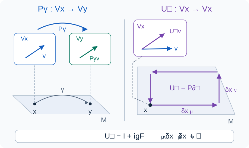
For the displayed orientation, transport first in the positive $\mu$ direction and then in the positive $\nu$ direction. Curvature measures the leading mismatch per area.

For a small rectangle traversed $+\mu ,+\nu ,-\mu ,-\nu$, with fixed distinct directions and no sum over them,

$$W_{\square }=I+ig{F}_{\mu \nu }\delta x^{\mu }\delta x^{\nu }+O(\delta x^3).$$

Reversing orientation changes the sign of the leading area term. The sign here is consistent with $D=\partial -igA$ and the transport equation above; it is not obtained by casually identifying transport operators with the derivative commutator.

An open transporter changes as $W^{\prime }(y,x)=U(y)W(y,x)U(x{)}^{-1}$. For a closed loop based at $x$, its trace is gauge invariant: this gives a Wilson loop. A flat connection has $F=0$ and is locally removable on sufficiently small simply connected patches. It can nevertheless have nontrivial global holonomy around noncontractible loops. The Aharonov–Bohm geometry provides an abelian example: accessible paths may enclose flux even when the field strength vanishes along those paths.

8.15 Electromagnetism and Yang–Mills dynamics

So far we have derived transformation rules and curvature. A physical theory also needs dynamics. In four-dimensional Minkowski spacetime, the usual gauge kinetic term for one nonabelian factor is

$${\mathcal{L}}_{\mathrm{gauge}}=-\frac{1}{2}\mathrm{tr}(F_{\mu \nu }{F}^{\mu \nu })=-\frac{1}{4}{F}_{\mu \nu }^a{F}^{a\mu \nu },$$

where the second equality uses our defining-representation trace normalization. Its action is invariant because $F$ transforms by conjugation. The antisymmetry in $\mu ,\nu$ and the spacetime metric contraction supply Lorentz invariance. This is the basic Yang–Mills kinetic term.

For electromagnetism, choose an electromagnetic coupling $e$ and a signed dimensionless charge $q$, so the physical charge is $eq$. Then

$$D_{\mu }={\partial }_{\mu }-ieq{A}_{\mu },{\psi }^{\prime }=e^{ieq\alpha }\psi ,A_{\mu }^{\prime }=A_{\mu }+{\partial }_{\mu }\alpha ,$$

and

$$F_{\mu \nu }={\partial }_{\mu }{A}_{\nu }-{\partial }_{\nu }{A}_{\mu },{\mathcal{L}}_{\mathrm{EM}}=-\frac{1}{4}{F}_{\mu \nu }{F}^{\mu \nu }.$$

For an electron, $q=-1$, hence this convention gives $D_{\mu }={\partial }_{\mu }+ie{A}_{\mu }$. A source using the opposite sign in $D$ must change its accompanying transformation conventions accordingly. Observable predictions do not depend on the convention chosen consistently.

Worked example 14: nonzero curvature from constant potentials

Take an $SU(2)$ gauge field on a patch with constant $A_x=a{t}_1$ and $A_y=b{t}_2$. All derivative terms vanish, but

$$F_{xy}=-igab[t_1,t_2]=gab{t}_3.$$

A spatially constant nonabelian connection need not be flat. The field strength arises entirely from noncommuting internal transport. In the abelian case constant potentials on a local patch would give zero curvature.

Expanding the Yang–Mills kinetic term reveals why nonabelian gauge fields interact with each other: $F$ contains both a derivative term linear in $A$ and a term quadratic in $A$. Squaring it produces terms cubic and quartic in the gauge potential. In pure abelian Maxwell theory the commutator vanishes, so no analogous photon self-interaction appears in the classical gauge kinetic term. Charged matter can still generate effective photon interactions through quantum loops.

Matter dynamics uses the same covariant derivative. For example, a scalar multiplet has

$${\mathcal{L}}_{\varphi }=(D_{\mu }\varphi {)}^{†}{D}^{\mu }\varphi -V({\varphi }^{†}\varphi ).$$

The representation determines which generators occur and therefore how the field couples. The gauge group alone does not choose the scalar potential, matter representations, or all permitted interaction coefficients.

The main QFT chapter takes the next steps: gauge fixing, quantization, propagators, running couplings, and scattering. Tong's Yang–Mills notes discuss this construction in more detail; that source sometimes absorbs the coupling into the connection, so compare definitions before comparing formulas.

8.16 Reading the Standard Model group and its matter table

The familiar local gauge structure is

$$G_{\mathrm{SM}}=SU(3{)}_c\times SU(2{)}_L\times U(1{)}_Y,{\mathfrak{g}}_{\mathrm{SM}}=\mathfrak{su}(3)\oplus \mathfrak{su}(2)\oplus \mathfrak{u}(1).$$

The subscript $c$ means color. The subscript $L$ says that Standard Model left-chiral fermions participate in weak doublets, whereas the right-chiral charged fermions are weak singlets. The subscript $Y$ denotes hypercharge. The weak $SU(2)$ is an internal group: its doublets are not spatial spinors simply because spatial spin also uses $SU(2)$ mathematics.

For a Dirac spinor, chirality is selected by $P_L=(1-{\gamma }^5)/2$ and $P_R=(1+{\gamma }^5)/2$. Helicity is spin projected along momentum. The two concepts align in specific ways for massless particles, but they are not interchangeable for massive particles. The labels in the table below refer to chirality.

We write an internal representation as $(R_c,R_L{)}_Y$, in that order, and use $Q=T_3+Y$. The entries $u_R,d_R,e_R$ below are actual right-chiral fields, not their left-chiral charge-conjugates. For one generation:

Field	Components	$(SU(3{)}_c,SU(2{)}_L{)}_Y$	Electric charges $Q$
$Q_L$	$(u_L,d_L{)}^T$, each with three colors	$(3,2{)}_{1/6}$	$2/3,-1/3$
$u_R$	right-chiral up quark, three colors	$(3,1{)}_{2/3}$	$2/3$
$d_R$	right-chiral down quark, three colors	$(3,1{)}_{-1/3}$	$-1/3$
$L_L$	$({\nu }_L,e_L{)}^T$	$(1,2{)}_{-1/2}$	$0,-1$
$e_R$	right-chiral charged lepton	$(1,1{)}_{-1}$	$-1$
$H$	complex scalar doublet $(H^{+},H^0{)}^T$	$(1,2{)}_{1/2}$	$1,0$

The fermion assignments repeat for three generations. The Higgs doublet is a single scalar multiplet, not a fourth fermion generation. The minimal renormalizable Standard Model has no ${\nu }_R$ and gives massless neutrinos; observed neutrino masses require additional ingredients such as higher-dimensional operators or new fields. The table's standard assignments and convention can be checked against Tong, section 5.1.

Worked example 15: read a product representation

The left quark doublet carries a color index $a=1,2,3$ and a weak index $i=1,2$. A transformation has the form

$$Q_L^{ai}⟼(U_c{)}^a{}_b(U_L{)}^i{}_j{e}^{i\beta /6}{Q}_L^{bj}.$$

The internal space is ${\mathbb{C}}^3\otimes {\mathbb{C}}^2$, with six components per generation. This is a tensor product because the two factors act on the same field through separate indices. Different group factors commute on that space: $U_c\otimes I_2$ commutes with $I_3\otimes U_L$. Within either nonabelian factor, transformations generally do not commute.

The parameter $\beta$ here is a local hypercharge parameter. To represent a compact circle with angle of period $2\pi$, use the integer-normalized charge $n=6Y$ and write $e^{in\theta }$, with $\beta =6\theta$. Fractional $Y$ is therefore a normalization convention, not a violation of the integer representation rule for $U(1)$.

The covariant derivative on any Standard Model multiplet is

$$D_{\mu }={\partial }_{\mu }-i{g}_s{G}_{\mu }^a{T}_c^a-ig{W}_{\mu }^i{T}_L^i-i{g}^{\prime }{B}_{\mu }Y.$$

Generators vanish when the field is a singlet of the corresponding factor. There are eight gluon gauge fields $G_{\mu }^a$, three weak gauge fields $W_{\mu }^i$, and one hypercharge gauge field $B_{\mu }$: $8+3+1=12$ algebra directions before electroweak symmetry breaking. These are species labels, not a count of physical polarization states. Right-chiral charged fermions still couple to hypercharge and, after mixing, to the photon and $Z$; weak singlet does not mean noninteracting.

8.17 How the photon emerges from electroweak mixing

Hypercharge is not electromagnetism. To see why, let the Higgs field have a potential with a minimum at $H^{†}H=v^2/2$. In a convenient gauge choose the vacuum representative

$$⟨H⟩=\frac{1}{\sqrt{2}}\left(\begin{array}{c}0\\ v\end{array}\right).$$

The lower component has $T_3=-1/2$ and $Y=+1/2$, so

$$(T_3+Y)⟨H⟩=0.$$

Thus the combination $Q=T_3+Y$ leaves the representative fixed. This identifies the unbroken electromagnetic generator. The usual phrase “electroweak symmetry breaking” describes this Higgs mechanism; a local gauge redundancy is not a physical symmetry that can be broken in the same sense as a global symmetry. The gauge-fixed vacuum language is a useful way to calculate the physical spectrum.

Worked example 16: obtain the neutral mixing matrix

Insert the constant Higgs representative into $(D_{\mu }H{)}^{†}{D}^{\mu }H$. With $T_i={\sigma }_i/2$ and $Y=1/2$, the gauge-field quadratic terms are

$$\frac{v^2}{8}\left[g^2\left((W_{\mu }^1{)}^2+(W_{\mu }^2{)}^2\right)+(g{W}_{\mu }^3-g^{\prime }{B}_{\mu }{)}^2\right],$$

where each square denotes a Lorentz contraction. Only one neutral combination appears in the massive term. Define

$$\tan {\theta }_W=\frac{g^{\prime }}{g},A_{\mu }=\sin {\theta }_W{W}_{\mu }^3+\cos {\theta }_W{B}_{\mu },$$ $$Z_{\mu }=\cos {\theta }_W{W}_{\mu }^3-\sin {\theta }_W{B}_{\mu },W_{\mu }^{\pm }=\frac{W_{\mu }^1\mp i{W}_{\mu }^2}{\sqrt{2}}.$$

Then $g{W}^3-g^{\prime }B=\sqrt{g^2+g^{\prime 2}}Z$. The orthogonal combination $A$ has no Higgs-generated mass and is the photon field. At tree level,

$$m_W=\frac{gv}{2},m_Z=\frac{v\sqrt{g^2+g^{\prime 2}}}{2},m_A=0.$$

Substitute the inverse mixing into the neutral part of the covariant derivative. The coefficient of $A_{\mu }$ is

$$g\sin {\theta }_W{T}_3+g^{\prime }\cos {\theta }_{W}Y=e(T_3+Y)=eQ,e=g\sin {\theta }_W=g^{\prime }\cos {\theta }_W.$$

This derives both the electric-charge operator and the electromagnetic coupling relation. The photon is a mixture of two original gauge fields, not simply a renamed hypercharge field. The formulas are tree-level relations; precision electroweak analysis requires renormalization and a specified scheme.

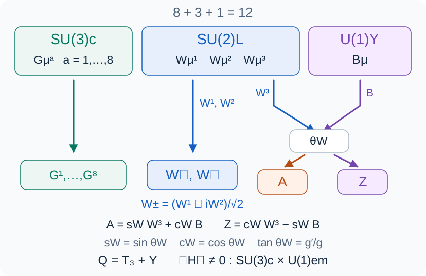
The product group acts on internal indices. Electroweak mixing combines $W^3$ and $B$, while color remains a separate gauge factor.

Worked example 17: recover the familiar electric charges

For $Q_L$, $T_3$ has eigenvalues $+1/2,-1/2$, while $Y=1/6$ multiplies both components. Thus $Q(u_L)=1/2+1/6=2/3$ and $Q(d_L)=-1/2+1/6=-1/3$. For $L_L$, $Y=-1/2$, giving $Q({\nu }_L)=0$ and $Q(e_L)=-1$. A weak singlet has $T_3=0$, so its electric charge equals its listed $Y$.

Before the Higgs mechanism the electroweak description has four massless gauge fields with two physical polarizations each and four real Higgs components: $8+4=12$ physical degrees of freedom. Afterwards there are three massive vector bosons with three polarizations each, one photon with two, and one Higgs scalar: $9+2+1=12$. This perturbative counting explains how the longitudinal vector modes arise without creating extra degrees of freedom. The eight gluons remain massless in the Lagrangian; confinement concerns their long-distance physical realization, not a Higgs mass term.

8.18 Global structure and what symmetry does not finish

Our earlier comparison of $SU(2)$ and $SO(3)$ prepares us for a subtlety in the Standard Model notation. Specifying a Lie algebra and its local couplings does not uniquely fix the global form of the gauge group.

Normalize the hypercharge circle by $n=6Y$, and set $\omega =e^{2\pi i/3}$. Consider the central element

$$z=\left(\omega I_3,-I_2,e^{i\pi /3}\right)\in SU(3)\times SU(2)\times U(1).$$

Its action on a field includes the phase $(e^{i\pi /3}{)}^{6Y}$. On $Q_L$ the total factor is $\omega (-1)e^{i\pi /3}=1$. On $L_L$ it is $(-1)e^{-i\pi }=1$; on $H$, $(-1)e^{i\pi }=1$. For $u_R,d_R,e_R$, it is respectively $\omega e^{4\pi i/3}=1$, $\omega e^{-2\pi i/3}=1$, and $e^{-2\pi i}=1$.

Consequently, the displayed matter fields cannot distinguish the subgroup generated by $z$, which is ${\mathbb{Z}}_6$. Their local representations are compatible with global forms

$$\frac{SU(3)\times SU(2)\times U(1)}{\Gamma },\Gamma \subseteq {\mathbb{Z}}_6,$$

including the trivial subgroup, ${\mathbb{Z}}_2$, ${\mathbb{Z}}_3$, or ${\mathbb{Z}}_6$. It is too strong to claim that the maximal quotient is uniquely established by the familiar particle table. These choices can differ in allowed line operators, bundles, and magnetic sectors despite sharing the local perturbative data discussed here. Tong, section 5.1.6 explains the qualification.

There are other unfinished tasks. Gauge invariance restricts interactions, but quantum consistency also demands cancellation of gauge anomalies. For a quick illustration, the mixed $SU(2{)}^{2}U(1)$ anomaly receives doublet contributions proportional to

$$3\left(\frac{1}{6}\right)+\left(-\frac{1}{2}\right)=0.$$

The factor three counts quark colors; the common doublet index $1/2$ has been suppressed. This is one cancellation, not a proof that every anomaly vanishes. A complete calculation includes cubic, mixed, and global anomalies, using consistent chirality conventions. In an all-left-chiral table, conjugating the right-chiral fields also conjugates their color representation and reverses hypercharge.

Gauge invariance permits Yukawa interactions such as ${\overline{L}}_{L}H{e}_R$: its hypercharges add to $+1/2+1/2-1=0$. It does not predict the Yukawa coupling's numerical value. Nor does the group name derive the Higgs potential, confinement, three generations, neutrino masses, dark matter, or gravity. Those require further dynamics, evidence, or extensions.

What we have achieved is a readable structure: group composition tells us how transformations combine; the Lie algebra tells us their local noncommutativity; representations tell us which fields carry which charges; a connection compares internal frames; curvature and invariant actions determine gauge dynamics. The frontiers chapter places that structure in the larger map of established physics and open questions.

8.19 Exercises with answers

Try each calculation before reading its answer. The aim is to reproduce the reasoning, not memorize a list of group names.

Exercise 1: a subgroup and a counterexample

Are the even integers a subgroup of $(\mathbb{Z},+)$? Are the positive real numbers a subgroup of the nonzero real numbers under multiplication?

Answer. Both are subgroups. Even integers include $0$, are closed under addition, and contain additive inverses. Positive real numbers include $1$, are closed under multiplication, and have positive reciprocals. Positivity fails to form a group under addition because $0$ and additive inverses are missing. Always specify the operation.

Exercise 2: inverses and the triangle

Using $r^3=s^2=e$ and $srs=r^{-1}$, find $(sr{)}^{-1}$ and show that $(sr{)}^2=e$.

Answer. The reverse-order rule gives $(sr{)}^{-1}=r^{-1}s$. Multiplying $srs=r^{-1}$ by $s$ on the left gives $rs=s{r}^{-1}$, and equivalently $sr=r^{-1}s$. Thus $(sr{)}^{-1}=sr$. Directly, $srsr=r^{-1}r=e$. The product $sr$ is a reflection, agreeing with its permutation $(13)$.

Exercise 3: a determinant and a dimension

Does $\mathrm{diag}(e^{i\alpha },e^{i\beta })$ lie in $SU(2)$? How many independent real parameters does $SU(4)$ have?

Answer. The diagonal matrix is always unitary, but is special unitary only if $\alpha +\beta$ is an integer multiple of $2\pi$. The dimension formula gives $4^2-1=15$. The defining representation has complex dimension four, a different number.

Exercise 4: compute a generator commutator

With $t_a={\sigma }_a/2$, evaluate $[t_2,t_3]$ and $\mathrm{tr}(t_3^2)$.

Answer. Since ${\sigma }_2{\sigma }_3=i{\sigma }_1$ and ${\sigma }_3{\sigma }_2=-i{\sigma }_1$, the commutator is $i{t}_1$. Also $t_3^2=I/4$, whose trace is $2/4=1/2$. Dropping the factors of two would change the structure constants or coupling normalization.

Exercise 5: which representations descend to $SO(3)$?

An irreducible $SU(2)$ representation has spin $j$ and dimension $2j+1$. A $2\pi$ rotation acts as $(-1{)}^{2j}I$. Which values of $j$ give representations of $SO(3)$?

Answer. A representation descends through the quotient by $\{I,-I\}$ only if $-I$ acts trivially. This occurs for integer $j=0,1,2,\dots$. Half-integer $j$ gives a nontrivial sign and does not descend. This is a global restriction invisible in the local commutator algebra alone.

Exercise 6: add two $U(1)$ charges

Two fields transform as $\varphi \mapsto e^{in\theta }\varphi$ and $\chi \mapsto e^{im\theta }\chi$. What are the charges of $\varphi \chi$ and ${\varphi }^{\ast }\chi$?

Answer. Multiplying the phases gives charges $n+m$ and $m-n$. Complex conjugation reverses a $U(1)$ charge. This is the abelian version of taking tensor products and conjugate representations, and it is how one quickly checks hypercharge neutrality of interaction terms.

Exercise 7: a pure gauge potential

Starting from $A_{\mu }=0$, transform by a smooth $U(x)$. What is $A_{\mu }^{\prime }$, and what is its curvature?

Answer. The potential is $A_{\mu }^{\prime }=-(i/g)({\partial }_{\mu }U)U^{-1}$. Its curvature vanishes because $F^{\prime }=UF{U}^{-1}=0$. A potential can be nonzero while its field strength is zero. This is a local statement for a smooth gauge transformation on the patch; global topology can obstruct one gauge choice covering an entire configuration.

Exercise 8: a small nonabelian loop

For $A_x=a{t}_1$, $A_y=b{t}_2$ constant, find transport around a small positively oriented $xy$ rectangle of area $S$ to leading order.

Answer. Section 8.15 gives $F_{xy}=gab{t}_3$, so $W_{\square }=I+i{g}^{2}abS{t}_3+\cdots$. The first nonzero effect is proportional to area, not to perimeter. Reversing the loop orientation reverses this leading term.

Exercise 9: count one fermion generation

Count the internal components in $Q_L,u_R,d_R,L_L,e_R$, without counting Lorentz-spinor components a second time. What changes if a sterile ${\nu }_R$ is added?

Answer. The count is $3\times 2+3+3+2+1=15$ Weyl fields per generation. A gauge-singlet ${\nu }_R$ adds one, giving sixteen, with assignment $(1,1{)}_0$. This count is neither the number of gauge generators nor the number of named particle flavors.

Exercise 10: test a Yukawa coupling

Check hypercharge neutrality of ${\overline{Q}}_{L}H{d}_R$ and ${\overline{Q}}_L\tilde{H}{u}_R$, where $\tilde{H}=i{\sigma }_2{H}^{\ast }$.

Answer. Conjugating $Q_L$ gives hypercharge $-1/6$. The first sum is $-1/6+1/2-1/3=0$. Since $\tilde{H}$ has $Y=-1/2$, the second is $-1/6-1/2+2/3=0$. Color indices contract between $\overline{3}$ and $3$; the weak doublet indices also contract to a singlet. Hypercharge neutrality is necessary, but all group factors must be checked.

Exercise 11: identify the electromagnetic generator

For a doublet with hypercharge $y$, find the two electric charges. For which $y$ is the lower component neutral?

Answer. The charges are $y+1/2$ and $y-1/2$. The lower component is neutral for $y=1/2$, the Higgs assignment. A neutral vacuum component allows the combination $T_3+Y$ to remain unbroken in the Higgs description.

Exercise 12: read what the group label leaves unspecified

Two theories have the same gauge algebra $\mathfrak{su}(3)\oplus \mathfrak{su}(2)\oplus \mathfrak{u}(1)$. Must they have the same particles, couplings, global group, and predictions?

Answer. No. They can have different matter representations, coupling values, scalar potentials, or global quotients, subject to consistency conditions such as anomaly cancellation. Even identical local field content can allow different global choices. The algebra constrains a theory; it is not the entire theory.

8.20 Glossary, reading map, and sources

Term	Meaning in this chapter
Group	A set with associative composition, identity, and inverses.
Abelian	Every pair of group elements commutes.
Action	A consistent rule by which a group transforms a set.
Homomorphism	A map preserving the composition law.
Kernel	Elements mapped to the identity transformation.
Faithful	Having a trivial kernel, so distinct group elements remain distinguishable.
Lie group	A smooth manifold with smooth group operations.
Lie algebra	Tangent space at the identity with its Lie bracket.
Generator	An infinitesimal transformation, often written in a Hermitian physics basis.
Structure constants	Coefficients expressing generator commutators in a chosen basis.
Representation	A group action by invertible linear maps on a vector space.
Irreducible	Having no nonzero proper invariant subspace.
Defining representation	The standard matrix action used to define a classical matrix group.
Adjoint representation	The action on the Lie algebra by conjugation.
Singlet	The trivial one-dimensional representation of the specified group.
Connection	A rule for comparing internal vectors at neighboring points.
Curvature	The failure of covariant derivatives, or infinitesimal transports, to commute.
Holonomy	The net transformation produced by transport around a closed path.
Gauge invariant	Unchanged by the allowed gauge transformations.
Gauge covariant	Transforming by a specified representation law.
Hypercharge	The $U(1{)}_Y$ generator, normalized here by $Q=T_3+Y$.
Chirality	The left or right Lorentz-spinor sector selected by ${\gamma }^5$, distinct from helicity for massive particles.

If a calculation stalls, return to the smallest concrete example. Test a composition on a triangle vertex. Test a matrix identity on the Pauli matrices. Test a gauge-transformation sign on a phase multiplying a constant field. Test a Standard Model charge on the lower component of the Higgs doublet. These checks connect abstract notation to operations we can perform explicitly.

The mathematical sources below establish the underlying definitions and theorems; the physics sources supply field-theory conventions and the Standard Model setting. The prose, worked examples, and diagrams in this article are original, with notation kept internally consistent rather than copied indiscriminately between references.

1. Pavel Etingof, Lie Groups and Lie Algebras I, MIT 18.745. Lectures 2–7 develop Lie groups, coverings, exponential maps, and brackets; Lecture 9 introduces representations. This is the mathematical continuation of sections 8.6–8.10.
2. Eckhard Meinrenken, Lie Groups and Lie Algebras, University of Toronto. A complementary account of matrix groups, exponential maps, and global versus local structure. Useful when the distinction between $SU(2)$ and $SO(3)$ needs a geometric second reading.
3. Peter Woit, Lie Groups and Representations, notes on Lie algebras, Columbia University, and representation generalities. These develop tangent-space conventions and the language of invariant subspaces, direct sums, and tensor products.
4. Hugh Osborn, Symmetries and Groups, University of Cambridge. Further group and representation theory for readers moving between mathematical and physics notation.
5. David Tong, The Standard Model, chapter 1: Symmetries, University of Cambridge. Section 1.3 connects Maxwell theory, Lie algebras, and Yang–Mills theory. It supports the gauge-theory framework used in sections 8.12–8.15.
6. David Tong, Gauge Theory, chapter 2: Yang–Mills Theory. A route onward to Wilson lines, nonabelian dynamics, and quantum gauge theory. Track where the coupling is included in the definition of the connection.
7. David Tong, The Standard Model, chapter 5: Electroweak Interactions. Sections 5.1–5.2 cover field assignments, anomaly constraints, global gauge-group choices, and electroweak mixing. Our ordering $(R_c,R_L{)}_Y$ places color first; the source uses its own ordering, so compare labels rather than column positions.

For the next stage within Open Physics Notes, continue with differential geometry for the geometric language, quantum field theory for dynamics and quantization, and frontiers of physics for the Standard Model's wider context and limitations.