Statistical physics

9.1 Foundations: From Microstates to Thermodynamics

Statistical physics is the art of predicting macroscopic laws from microscopic uncertainty. We never know the exact $1 0^{23}$ -body state; instead we organize ignorance into ensembles whose averages reproduce temperature, pressure, magnetization, and friends. This section builds the core: microstates vs macrostates, the fundamental postulate, the three standard ensembles, and the thermodynamic limit. We also show how the information-theoretic view turns “maximum entropy” into the unique engine behind the familiar distributions.

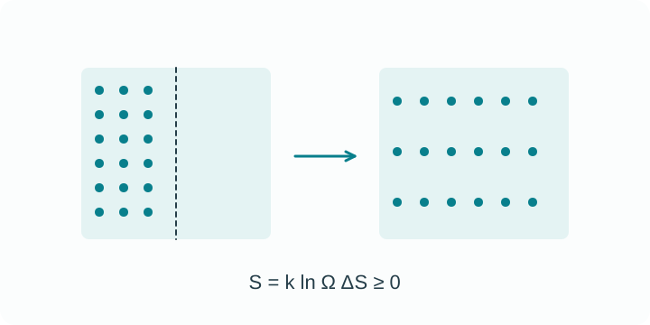
A gas initially confined to half a container expands into the whole isolated container. More accessible microstates correspond to larger entropy.

9.1.1 Microstates, macrostates, and phase space

A microstate is a complete specification of the system’s degrees of freedom. For $N$ classical point particles, it is a point in $6 N$ -dimensional phase space with coordinates

Γ \equiv (r_{1}, \dots, r_{N}; p_{1}, \dots, p_{N})

A macrostate is defined by a few bulk variables, e.g., $(E, V, N)$ for an isolated gas. Many microstates map to the same macrostate. Counting how many leads to entropy.

Liouville’s theorem states that Hamiltonian flow is incompressible in phase space, so volume elements are preserved along trajectories. This makes uniform distributions over energy shells dynamically consistent.

9.1.2 Fundamental postulate and Boltzmann’s principle

Fundamental postulate. For an isolated system with fixed $(E, V, N)$ at equilibrium, all microstates compatible with these constraints are equally likely.

Let $Ω (E, V, N)$ be the number of microstates with energies in $[E, E + δ E]$ for a small but macroscopic $δ E$ . Then the entropy is

S (E, V, N) = k_{B} ln Ω (E, V, N)

Thermodynamic temperature follows from

\frac{1}{T} = (\frac{\partial S}{\partial E})_{V, N}

and pressure and chemical potential are

\frac{p}{T} = (\frac{\partial S}{\partial V})_{E, N}, - \frac{μ}{T} = (\frac{\partial S}{\partial N})_{E, V}

For weakly interacting subsystems $A$ and $B$ , additivity of $S$ at fixed total $E$ yields the equilibrium condition $T_{A} = T_{B}$ by maximizing $S_{A} (E_{A}) + S_{B} (E_{B})$ subject to $E_{A} + E_{B} = E$ .

9.1.3 Thermodynamic limit, extensivity, and concavity

Define the thermodynamic limit as $N \to \infty$ , $V \to \infty$ with $n = N / V$ fixed. In this limit:

Entropy becomes extensive: $S (λ E, λV, λ N) \approx λ S (E, V, N)$
$S$ is concave in its natural variables, ensuring stability and positive heat capacities where appropriate
Fluctuations of intensive variables shrink like $1/ N$ , making thermodynamics sharp

Short-range interactions guarantee ensemble equivalence; long-range cases (self-gravity, unscreened Coulomb) can violate additivity and need care.

9.1.4 Microcanonical ensemble

The microcanonical probability density is uniform with respect to the invariant energy-shell measure induced by Liouville measure, rather than Euclidean hypersurface area. Here $ω (E, V, N) = \int d Γ δ (H (Γ) - E)$ is the density of states, distinct from the finite-shell count $Ω ≃ ω δ E$ for a fixed narrow energy width:

ρ_{mc} (Γ) = \frac{1}{ω ( E , V , N )} δ (H (Γ) - E)

Expectations are

⟨ A ⟩_{mc} = \frac{1}{ω} \int d Γ A (Γ) δ (H (Γ) - E)

Maximizing $S = k_{B} ln Ω$ subject to constraints reproduces thermodynamic relations. For many systems this is the conceptual anchor; in practice the canonical ensemble is often easier to compute with and becomes equivalent at large $N$ .

9.1.5 Canonical ensemble via a heat bath

Place system $S$ weakly coupled to a huge reservoir $R$ with fixed $E_{tot}$ . The probability that $S$ is found in microstate $i$ with energy $E_{i}$ is proportional to the number of reservoir states at energy $E_{tot} - E_{i}$ :

P (i) \propto Ω_{R} (E_{tot} - E_{i}) \approx exp [\frac{1}{k _{B}} S_{R} (E_{tot}) - \frac{E _{i}}{k _{B} T}] \propto e^{- β E_{i}}

with inverse temperature $β \equiv 1/ (k_{B} T)$ . Normalize to get

P (i) = \frac{e ^{- β E_{i}}}{Z}, Z (β, V, N) \equiv i \sum e^{- β E_{i}}

$Z$ is the partition function. Thermodynamic potentials follow:

F (T, V, N) \equiv - k_{B} T ln Z

U = ⟨ E ⟩ = - \frac{\partial}{\partial β} ln Z

S = - (\frac{\partial F}{\partial T})_{V, N} = k_{B} (ln Z + β U)

Energy fluctuations satisfy

⟨(Δ E)^{2} ⟩ = k_{B} T^{2} C_{V}

so relative fluctuations scale as $1/ N$ for normal systems.

9.1.6 Grand canonical ensemble: exchanging particles

If both energy and particles exchange with a reservoir, the probability of microstate $i$ with $(E_{i}, N_{i})$ is

P (i) = \frac{e ^{- β (E_{i} - μ N_{i})}}{Ξ}

with grand partition function

Ξ (β, V, μ) \equiv N = 0 \sum \infty i \in N \sum e^{- β (E_{i} - μ N)}

Define the grand potential

Φ_{G} (T, V, μ) \equiv - k_{B} T ln Ξ

Then

p = - (\frac{\partial Φ _{G}}{\partial V})_{T, μ}, N = - (\frac{\partial Φ _{G}}{\partial μ})_{T, V}, S = - (\frac{\partial Φ _{G}}{\partial T})_{V, μ}

Fluctuations:

⟨(Δ N)^{2} ⟩ = k_{B} T (\frac{\partial N}{\partial μ})_{T, V}

and energy–number covariances come from mixed derivatives of $ln Ξ$ .

9.1.7 Legendre transforms and thermodynamic potentials

Thermodynamics is organized by Legendre transforms that swap natural variables:

$S = S (E, V, N)$
$F = U - TS$ with natural variables $(T, V, N)$
$G = F + p V$ with $(T, p, N)$
$H = U + p V$ with $(S, p, N)$
$Φ_{G} = F - μ N$ with $(T, V, μ)$

Maxwell relations follow from equality of mixed partial derivatives, e.g.,

(\frac{\partial S}{\partial V})_{T} = (\frac{\partial p}{\partial T})_{V}

9.1.8 Information-theoretic foundation (Jaynes view)

Let ${p_{i}}$ be probabilities over microstates. Maximize the Shannon entropy

S [p] \equiv - k_{B} i \sum p_{i} ln p_{i}

subject to known constraints. With only normalization and mean energy fixed, Lagrange multipliers give

p_{i} = \frac{e ^{- β E_{i}}}{Z}

With energy and particle number constraints, one obtains the grand canonical form $p_{i} \propto e^{- β (E_{i} - μ N_{i})}$ . Thus ensembles are the least biased distributions compatible with macroscopic data.

Relative entropy $D (p ∥ q) = \sum p_{i} ln (p_{i} / q_{i}) \geq 0$ measures distance to a prior $q$ . Many fluctuation theorems and linear-response results are compact in this language.

9.1.9 Large deviations, concentration, and ensemble equivalence

For $N ≫ 1$ , probabilities concentrate exponentially near thermodynamic values. If $A$ is an additive observable,

P (\frac{A}{N} \approx a) \sim e^{- N I (a)}

with a rate function $I (a) \geq 0$ that vanishes at the equilibrium value. Under standard convexity conditions:

Microcanonical, canonical, and grand canonical ensembles are equivalent in the thermodynamic limit
Nonconcavities signal phase coexistence; Maxwell constructions repair them at the level of thermodynamic potentials

9.1.10 Worked mini-examples

(a) Two-level system
Energy levels $0$ and $ϵ$ for $N$ noninteracting sites. Canonical partition function per site

z = 1 + e^{- β ϵ}

Total $Z = z^{N}$ . Average energy $U = N ϵ / (e^{β ϵ} + 1)$ and heat capacity shows a Schottky peak near $k_{B} T \sim ϵ$ .

(b) Quantum harmonic oscillator
Single oscillator with $E_{n} = (n + \frac{1}{2}) ℏ ω$ gives

Z = \frac{e ^{- β ℏ ω /2}}{1 - e ^{- β ℏ ω}}

Average energy $U = \frac{ℏ ω}{2} + \frac{ℏ ω}{e ^{β ℏ ω} - 1}$ tends to $k_{B} T$ at high $T$ (equipartition) and to $ℏ ω /2$ at $T \to 0$ .

(c) Coin toss and Stirling
For $N$ independent fair coins, the multiplicity of $k$ heads is $(k N) \approx exp [N H (k / N)] / 2 π N x (1 - x)$ with $x = k / N$ and binary entropy $H (x) = - x ln x - (1 - x) ln (1 - x)$ . This is the large-deviation archetype.

(d) Ideal gas microcanonical temperature
For a classical ideal gas, counting states yields

Ω (E, V, N) \propto \frac{V ^{N} E ^{\frac{3 N}{2} - 1}}{N ! Γ ( \frac{3 N}{2} )}

so, at fixed energy-shell width, $S = k_{B} ln Ω$ gives $U = (\frac{3 N}{2} - 1) k_{B} T$ and $p V = N k_{B} T$ . In the thermodynamic limit, $U ≃ \frac{3}{2} N k_{B} T$ .

(e) Canonical fluctuations
Show $⟨(Δ E)^{2} ⟩ = k_{B} T^{2} C_{V}$ by taking $\partial_{β}^{2} ln Z$ and relate the heat capacity to curvature of $ln Z$ .

9.1.11 Minimal problem kit

Starting from $S = k_{B} ln Ω$ , derive $1/ T = (\partial S / \partial E)_{V, N}$ and $p / T = (\partial S / \partial V)_{E, N}$
Derive the canonical ensemble by maximizing $S [p]$ with constraints $\sum p_{i} = 1$ and $\sum p_{i} E_{i} = U$
Show that $F = - k_{B} T ln Z$ implies $S = - \partial F / \partial T$ and $p = - \partial F / \partial V$
For a classical ideal gas, compute $Ω (E, V, N)$ up to a constant using phase-space volume and obtain the Sackur–Tetrode entropy
Prove $⟨(Δ N)^{2} ⟩ = k_{B} T (\partial N / \partial μ)_{T, V}$ in the grand canonical ensemble
Discuss when ensemble equivalence fails and give a physical example with long-range forces

9.2 Partition Functions & Thermodynamic Potentials

Partition functions are the generators of everything thermodynamic. Once you have $Z$ or $Ξ$ or the $N pT$ analogue, derivatives give you $U, p, S, μ$ and all the response coefficients. This section builds the canonical and grand-canonical machinery, adds the isothermal–isobaric ensemble, and shows how Legendre transforms and saddle points tie them back to microcanonical entropy. Worked examples anchor the formulas.

9.2.1 Canonical partition function and cumulants

For fixed $(T, V, N)$ the canonical weights are $P (i) \propto e^{- β E_{i}}$ with

Z (β, V, N) \equiv i \sum e^{- β E_{i}}

Helmholtz free energy

F (T, V, N) \equiv - k_{B} T ln Z

Standard derivatives

U \equiv ⟨ E ⟩ = - \frac{\partial}{\partial β} ln Z

S = - (\frac{\partial F}{\partial T})_{V, N} = k_{B} (ln Z + β U)

p = - (\frac{\partial F}{\partial V})_{T, N}

Energy cumulants follow from derivatives of $ln Z$ with respect to $β$ . For instance

⟨(Δ E)^{2} ⟩ = \frac{\partial ^{2}}{\partial β ^{2}} ln Z = k_{B} T^{2} C_{V}

Generalized forces for a control parameter $λ$ that enters $H (λ)$ obey

(\frac{\partial F}{\partial λ})_{T, V, N} = ⟨ \frac{\partial H}{\partial λ} ⟩

Examples: $M = - (\partial F / \partial B)_{T, V, N}$ for a magnetic field $B$ and $p = - (\partial F / \partial V)_{T, N}$ for volume.

9.2.2 Grand partition function, fugacity, and pressure

When particle number fluctuates at fixed $(T, V, μ)$

Ξ (β, V, μ) \equiv N = 0 \sum \infty i \in N \sum e^{- β (E_{i} - μ N)}

Define the grand potential

Φ_{G} (T, V, μ) \equiv - k_{B} T ln Ξ

Thermodynamics in this ensemble is compact

p = - (\frac{\partial Φ _{G}}{\partial V})_{T, μ}

N = - (\frac{\partial Φ _{G}}{\partial μ})_{T, V}

S = - (\frac{\partial Φ _{G}}{\partial T})_{V, μ}

It is common to use the fugacity $z \equiv e^{β μ}$ . Number fluctuations and compressibility are linked by

⟨(Δ N)^{2} ⟩ = k_{B} T (\frac{\partial N}{\partial μ})_{T, V}

For a uniform ideal gas one finds the handy identity $p V = k_{B} T ln Ξ$ .

9.2.3 Isothermal–isobaric ensemble and Gibbs free energy

Many experiments hold $(T, p, N)$ fixed. The isothermal–isobaric partition function is the Laplace transform of $Z$ over $V$ , with a fixed reference volume $V_{0}$ making it dimensionless:

Δ (β, p, N) \equiv \int_{0}^{\infty} \frac{d V}{V _{0}} e^{- βp V} Z (β, V, N)

Its thermodynamic potential is the Gibbs free energy

G (T, p, N) \equiv - k_{B} T ln Δ

Then

(\frac{\partial G}{\partial p})_{T, N} = V, (\frac{\partial G}{\partial T})_{p, N} = - S, (\frac{\partial G}{\partial N})_{T, p} = μ

Fluctuations of $V$ at fixed $(T, p, N)$ are generated by derivatives of $ln Δ$ .

9.2.4 Legendre structure and microcanonical link

Canonical and grand-canonical ensembles are Laplace transforms of the microcanonical state count

Z (β, V, N) = \int d E ω (E, V, N) e^{- βE}

For large systems the integral is dominated by a saddle point $E^{*}$ with $\partial_{E} ln ω ∣_{E^{*}} = β$ , i.e., $1/ T = \partial S / \partial E$ . Evaluating at the saddle yields the Legendre relation

F (T, V, N) = U - TS

Similarly, the grand-canonical transform over both $E$ and $N$ yields

Φ_{G} (T, V, μ) = U - TS - μ N

These are the reasons thermodynamic potentials are Legendre transforms of $S$ .

9.2.5 Ideal classical gas in the canonical ensemble

Take $N$ indistinguishable particles of mass $m$ with Hamiltonian $H = \sum p_{i}^{2} /2 m$ and ignore interactions. The canonical partition function factorizes into a translational part

Z (β, V, N) = \frac{1}{N !} [\frac{V}{λ _{T}^{3}}]^{N}

with thermal wavelength

λ_{T} \equiv \frac{2 π ℏ ^{2}}{m k _{B} T}

Then

F = - k_{B} T ln Z = - N k_{B} T [ln (\frac{V}{N λ _{T}^{3}}) + 1]

Equation of state follows immediately

p V = N k_{B} T

Entropy is the Sackur–Tetrode form

S = N k_{B} [ln (\frac{V}{N λ _{T}^{3}}) + \frac{5}{2}]

and the internal energy is $U = \frac{3}{2} N k_{B} T$ with $C_{V} = \frac{3}{2} N k_{B}$ . The $1/ N!$ cures the Gibbs paradox by enforcing indistinguishability.

9.2.6 Quantum ideal gases via the cluster expansion

For noninteracting bosons or fermions with one-particle energies ${ϵ_{α}}$

ln Ξ = \mp α \sum ln (1 \mp z e^{- β ϵ_{α}})

upper sign for bosons, lower for fermions. Occupations are

⟨ n_{α} ⟩ = \frac{1}{z ^{- 1} e ^{β ϵ_{α}} \mp 1}

In the continuum limit one replaces $\sum_{α} \to \int d ϵ g (ϵ)$ to obtain thermodynamics of photon, phonon, or electron gases. Interactions can be included perturbatively via virial or cluster expansions that correct $ln Ξ$ by coefficients $B_{2}, B_{3}, \dots$ .

9.2.7 Generalized forces and response matrices

If a classical Hamiltonian depends linearly on external controls $λ = (λ_{1}, \dots)$ , the matrix of second derivatives of $F$ gives the covariance response below. The same equal-time form applies to quantum observables commuting with the Hamiltonian. Nonlinear coupling requires an additional explicit derivative term, and noncommuting quantum observables require the imaginary-time Kubo correlation:

χ_{ab} \equiv - (\frac{\partial ^{2} F}{\partial λ _{a} \partial λ _{b}})_{T, V, N} = β ⟨ Δ X_{a} Δ X_{b} ⟩

where $X_{a} \equiv - \partial H / \partial λ_{a}$ is the conjugate observable. Examples include magnetic susceptibility, compressibility, and heat capacities. Mixed derivatives encode Maxwell relations, e.g., $(\partial S / \partial V)_{T, N} = (\partial p / \partial T)_{V, N}$ .

9.2.8 Ising-like lattice systems and counting practice

For a finite lattice with spins $s_{i} = \pm 1$ and Hamiltonian $H = - J \sum_{⟨ ij ⟩} s_{i} s_{j} - h \sum_{i} s_{i}$ the canonical partition function is

Z (β, h) = {s} \sum exp β J ⟨ ij ⟩ \sum s_{i} s_{j} + β h i \sum s_{i}

While exact evaluation is hard beyond 1D, derivatives of $ln Z$ still define magnetization $M = (\partial ln Z / \partial (β h))$ and susceptibility $χ = \partial M / \partial h$ . Mean-field or transfer-matrix approaches approximate $Z$ systematically.

9.2.9 Gibbs–Duhem and extensivity checks

For an extensive system with $U (S, V, N)$ homogeneous of degree one, Euler’s relation holds

U = TS - p V + μ N

Differentiating yields the Gibbs–Duhem equation

S d T - V d p + N d μ = 0

This is a consistency check for any equation of state you derive from a partition function.

9.2.10 Laplace tricks, saddle points, and when ensembles match

Because $Z$ and $Δ$ are Laplace transforms, large- $N$ thermodynamics follows from their leading saddle. Concavity of $S (E, V, N)$ guarantees equivalence of ensembles. At first-order transitions $Z$ develops multiple competing saddles; Legendre transforms pick the convex envelope, and fluctuations become non-Gaussian in finite systems.

9.2.11 Worked mini-examples

(a) $N pT$ ideal gas

Compute $Δ$ for the ideal gas using $Z = (V / λ_{T}^{3})^{N} / N!$ to show

Δ = \frac{1}{V _{0} λ _{T}^{3 N} ( βp ) ^{N + 1}}

and verify $G = N k_{B} T ln (βp λ_{T}^{3}) + k_{B} T ln (βp V_{0})$ and $V = (\partial G / \partial p)_{T, N} = (N + 1) k_{B} T / p$ . For large $N$ , the relative $1/ N$ correction vanishes and $V ≃ N k_{B} T / p$ .

(b) Pressure from $Z$ via the virial

For a classical interacting gas with pair potential $u (r)$ , show that $p = N k_{B} T / V - \frac{2 π n ^{2}}{3} \int_{0}^{\infty} d r r^{3} u^{'} (r) g (r)$ using $p = - (\partial F / \partial V)_{T, N}$ and a uniform scaling argument, where $n = N / V$ and $g (r)$ is the pair distribution.

(c) Number fluctuations and compressibility

In the grand ensemble, verify $⟨(Δ N)^{2} ⟩ = k_{B} T (\partial N / \partial μ)_{T, V}$ and relate to the isothermal compressibility $κ_{T} = \frac{1}{n ^{2}} (\partial n / \partial μ)_{T}$ .

(d) Microcanonical ↔ canonical

Starting from $Z ≃ \int (d E / δ E) exp [S (E) / k_{B} - βE]$ , perform a quadratic expansion of $S (E)$ about $E^{*}$ to obtain Gaussian energy fluctuations with variance $k_{B} T^{2} C_{V}$ .

(e) Two-level system free energy

For $N$ independent two-level sites with energies $0$ and $ϵ$ , compute $Z = (1 + e^{- β ϵ})^{N}$ , then $F$ , $S$ , and $C_{V}$ and locate the Schottky peak.

9.2.12 Minimal problem kit

Derive all canonical relations for $U, S, p$ starting from $F = - k_{B} T ln Z$ and verify the Maxwell relation $(\partial S / \partial V)_{T, N} = (\partial p / \partial T)_{V, N}$
Show that in the grand ensemble, $p V = k_{B} T ln Ξ$ for an ideal gas and obtain $N$ and $S$ from derivatives of $ln Ξ$
Compute the isothermal–isobaric partition function for a classical harmonic solid treated as $3 N$ independent oscillators and extract $G (T, p, N)$ in the limit of weak compressibility
Using $ln Ξ = \mp \sum_{α} ln (1 \mp z e^{- β ϵ_{α}})$ , recover the Bose–Einstein and Fermi–Dirac distributions and the classical limit when $z ≪ 1$
From extensivity, prove Euler’s relation $U = TS - p V + μ N$ and then the Gibbs–Duhem equation, and test them on the ideal gas results above

9.3 Classical Ideal Gas & Equipartition

The classical ideal gas is the training montage of statistical physics: you learn to count states, take derivatives of $ln$ partition functions, and watch macroscopic laws fall out like it’s nothing. We derive the Maxwell–Boltzmann distribution, prove equipartition, recover $p V = N k_{B} T$ , and build intuition for adiabats, sound speed, and when the classical picture breaks (hello, $λ_{T}$ ).

9.3.1 Canonical counting recap and the ideal-gas Z

For $N$ indistinguishable point particles of mass $m$ in volume $V$ with Hamiltonian $H = \sum_{i = 1}^{N} p_{i}^{2} /2 m$ , the canonical partition function factorizes:

Z (β, V, N) = \frac{1}{N !} [\frac{V}{λ _{T}^{3}}]^{N}

with thermal wavelength

λ_{T} \equiv \frac{2 π ℏ ^{2}}{m k _{B} T}

Thermodynamics then follows immediately:

F = - N k_{B} T [ln (\frac{V}{N λ _{T}^{3}}) + 1], U = \frac{3}{2} N k_{B} T, p V = N k_{B} T

Heat capacities:

C_{V} = (\frac{\partial U}{\partial T})_{V, N} = \frac{3}{2} N k_{B}, C_{p} = C_{V} + N k_{B} = \frac{5}{2} N k_{B}, γ \equiv \frac{C _{p}}{C _{V}} = \frac{5}{3}

Entropy is the Sackur–Tetrode form:

S = N k_{B} [ln (\frac{V}{N λ _{T}^{3}}) + \frac{5}{2}]

The $1/ N!$ kills the Gibbs paradox by encoding indistinguishability.

9.3.2 Maxwell–Boltzmann distribution (velocities, speeds, energies)

Each momentum component is Gaussian:

f (p_{x}) = \frac{β}{2 πm} exp (- \frac{β p _{x}^{2}}{2 m})

Equivalently, each velocity component is Gaussian with variance $⟨ v_{x}^{2} ⟩ = k_{B} T / m$ . The speed distribution (radial in velocity space) is

f (v) = 4 π (\frac{m}{2 π k _{B} T})^{3/2} v^{2} exp (- \frac{m v ^{2}}{2 k _{B} T})

Useful moments:

v_{mp} = \frac{2 k _{B} T}{m}, ⟨ v ⟩ = \frac{8 k _{B} T}{πm}, v_{rms} = \frac{3 k _{B} T}{m}

The kinetic energy distribution is $χ^{2}$ -like with $3$ degrees of freedom:

f (E) = \frac{2}{π} \frac{1}{( k _{B} T ) ^{3/2}} E e^{- E / k_{B} T}, ⟨ E ⟩ = \frac{3}{2} k_{B} T

9.3.3 Equipartition theorem

Statement. Every quadratic degree of freedom in the Hamiltonian contributes $\frac{1}{2} k_{B} T$ to the mean energy.

Sketch of proof (canonical, integration by parts). If $H$ contains a term $α x^{2}$ , then

⟨ x \partial H / \partial x ⟩ = k_{B} T

For $H = \sum p_{i}^{2} /2 m + \dots$ , each quadratic $p_{i}^{2} /2 m$ gives $⟨ p_{i}^{2} /2 m ⟩ = \frac{1}{2} k_{B} T$ . A monatomic gas has $3 N$ translational momenta → $U = \frac{3}{2} N k_{B} T$ .

When it fails (and why that’s good). Classical equipartition fails when quantized rotations or vibrations have level spacings larger than $k_{B} T$ , even if the Hamiltonian is quadratic. Their thermal contributions “freeze out.” This explains the drop of specific heats at low $T$ and the range of validity of Dulong–Petit.

9.3.4 Kinetic-theory

From elastic impacts on a wall, the pressure can be written

p = \frac{2}{3} \frac{U}{V}

Combine with $U = \frac{3}{2} N k_{B} T$ to get $p V = N k_{B} T$ . More generally, for pairwise interactions $u (r)$ the virial theorem yields

p V = N k_{B} T + \frac{1}{3} ⟨ i < j \sum r_{ij} \cdot F_{ij} ⟩

The ideal gas has $F_{ij} = 0$ , so the second term vanishes.

9.3.5 Adiabats, sound speed, and quick thermodynamic moves

For a reversible adiabatic change ( $d Q = 0$ ) in a monatomic ideal gas,

p V^{γ} = const, T V^{γ - 1} = const, T^{γ} p^{1 - γ} = const

with $γ = 5/3$ . The speed of sound (small adiabatic density waves) is

c_{s} = γ \frac{k _{B} T}{m}

For mixtures, replace $m$ by the mean molecular mass and $γ$ by the appropriate ratio of heat capacities.

9.3.6 External fields: barometric formula and separability

In a uniform gravitational field $U (z) = m g z$ , the one-body Boltzmann weight factorizes:

n (z) \propto e^{- β m g z}, n (z) = n (0) e^{- z / H}, H \equiv \frac{k _{B} T}{m g}

The momentum and position parts separate, so kinetic-energy results (equipartition, MB speeds) survive untouched.

9.3.7 Transport in one screen: mean free path and friends

For hard spheres of diameter $d$ at number density $n$ , the mean free path is

ℓ ≃ \frac{1}{2 π d ^{2} n}

Using typical speed $\overset{v}{ˉ} \sim ⟨ v ⟩$ ,

D \sim \frac{1}{3} \overset{v}{ˉ} ℓ, η \sim \frac{1}{3} nm \overset{v}{ˉ} ℓ, κ \sim \frac{1}{3} n C_{V}^{per particle} \overset{v}{ˉ} ℓ

These kinetic-theory scalings are remarkably good for dilute gases; real cross sections and mixtures refine the prefactors.

9.3.8 Validity of the classical picture

Classical, nondegenerate behavior requires the diluteness parameter to be small:

n λ_{T}^{3} ≪ 1

If $n λ_{T}^{3} ≳ 1$ (low $T$ or high $n$ ), quantum statistics kicks in: bosons want Bose–Einstein, fermions go Pauli, and the MB distribution is no longer the move.

9.3.9 Beyond monatomic: what equipartition counts

For a rigid linear diatomic at intermediate $T$ :

$3$ translational + $2$ rotational quadratic modes → $f = 5$ effective d.o.f., so $C_{V} \approx \frac{5}{2} N k_{B}$ , $γ \approx 7/5$
Vibrations add $2$ more quadratic modes but only when $k_{B} T$ exceeds the vibrational quantum spacing; otherwise they’re frozen

Moral: count only the modes that are active at your $T$ .

9.3.10 Worked mini-examples

(a) RMS speed for air at room $T$

For $N_{2}$ with $m \approx 28 u$ at $T = 300 K$ ,

v_{rms} = \frac{3 k _{B} T}{m}

Plug numbers to get a few hundred $m/s$ ; compare to $v_{mp}$ and $⟨ v ⟩$ .

(b) Adiabatic compression

A monatomic gas is compressed from $(p_{1}, V_{1})$ to $(p_{2}, V_{2})$ adiabatically. Use $p V^{γ} = const$ to find $T_{2} / T_{1} = (V_{1} / V_{2})^{γ - 1}$ .

(c) Barometric scale height of helium

For He at $T = 300 K$ , compute $H = k_{B} T / (m g)$ and compare to $N_{2}$ to see the mass dependence pop.

(d) Mean free path at STP

Take $d \approx 0.3 nm$ , $n \approx 2.5 \times 1 0^{25} m^{- 3}$ ; estimate $ℓ$ and comment on why smells diffuse fast.

(e) Equipartition sanity check

Show directly from $\int d p p^{2} e^{- β p^{2} /2 m}$ that $⟨ p^{2} /2 m ⟩ = \frac{1}{2} k_{B} T$ and extend to three components.

9.3.11 Minimal problem kit

Starting from $f (v)$ , derive $v_{mp}$ , $⟨ v ⟩$ , and $v_{rms}$
Prove the equipartition identity $⟨ x \partial H / \partial x ⟩ = k_{B} T$ for a quadratic coordinate and apply it to $p^{2} /2 m$
Derive $p = \frac{2}{3} U / V$ via wall-collision counting and recover $p V = N k_{B} T$
For a linear diatomic with rotational constant $B$ , estimate the temperature where rotations “turn on” by comparing $k_{B} T$ to $ℏ^{2} / (2 I)$
Check the classicality criterion for a cold atomic gas of density $n$ and temperature $T$ : compute $n λ_{T}^{3}$ and discuss when quantum statistics is required

9.4 Fluctuations & the Fluctuation–Response Principle

Macroscopic laws look crisp because relative fluctuations scale like $1/ N$ —until they don’t. This section organizes what fluctuates, how much, and why responses equal fluctuations. We connect the canonical, grand-canonical, and isothermal–isobaric ensembles; introduce static fluctuation–dissipation relations; link pair correlations to compressibility; and preview what breaks near critical points.

9.4.1 Energy and number: the two flagship variances

Canonical (fixed $T, V, N$ ):

⟨(Δ E)^{2} ⟩ = \frac{\partial ^{2}}{\partial β ^{2}} ln Z = k_{B} T^{2} C_{V}

Relative size shrinks as $⟨(Δ E)^{2} ⟩^{1/2} / U \sim 1/ N$ for normal systems.

Grand canonical (fixed $T, V, μ$ ):

⟨(Δ N)^{2} ⟩ = k_{B} T (\frac{\partial N}{\partial μ})_{T, V}

Equivalently, in terms of density $n = N / V$ and isothermal compressibility $κ_{T} \equiv - \frac{1}{V} (\frac{\partial V}{\partial p})_{T, N}$ ,

⟨(Δ N)^{2} ⟩ = N k_{B} T n κ_{T}

for a single-component fluid where $d n = χ_{μ} d μ$ and standard thermodynamic identities have been used.

9.4.2 Volume fluctuations at fixed pressure

Holding $(T, p, N)$ fixed, the isothermal–isobaric partition function $Δ$ generates

⟨(Δ V)^{2} ⟩ = - k_{B} T (\frac{\partial V}{\partial p})_{T, N} = k_{B} T V κ_{T}

Again, fluctuation = response: compressibility measures how much $V$ wiggles when $p$ nudges; that same coefficient sets the equilibrium variance.

9.4.3 Static fluctuation–response in one line

Let a control $λ$ couple to a source-independent observable $X$ via $H \to H - λ X$ (so $X = - \partial H / \partial λ$ ). In a classical canonical ensemble, or for a quantum observable commuting with the Hamiltonian,

χ_{XX} \equiv (\frac{\partial ⟨ X ⟩}{\partial λ})_{T, V, N} = β ⟨(Δ X)^{2} ⟩

Special cases:

For energy, $\partial U / \partial β = - ⟨(Δ E)^{2} ⟩$ and $\partial U / \partial T = C_{V}$ give $⟨(Δ E)^{2} ⟩ = k_{B} T^{2} C_{V}$ . Here inverse temperature is the conjugate parameter in the Boltzmann weight; varying it is distinct from the fixed-temperature source $λ$ above.
$X = N$ in the grand ensemble gives $(\partial N / \partial μ)_{T, V} = β ⟨(Δ N)^{2} ⟩$

Positivity of variances $\Rightarrow$ stability: $C_{V} \geq 0$ , $κ_{T} \geq 0$ in ensembles with fixed $T$ .

9.4.4 Correlations, structure factor, and the compressibility sum rule

Define the microscopic density $\overset{n}{^} (r) = \sum_{i} δ (r - r_{i})$ , the pair correlation $g (r)$ , and the static structure factor

S (k) \equiv \frac{1}{N} ⟨ δ \overset{n}{^}_{k} δ \overset{n}{^}_{- k} ⟩, δ \overset{n}{^}_{k} \equiv \int d^{3} r e^{- i k \cdot r} [\overset{n}{^} (r) - n]

In a uniform fluid,

S (k) = 1 + n \int d^{3} r e^{- i k \cdot r} [g (r) - 1]

Taking $k \to 0$ connects microscopic correlations to macroscopic response:

S (0) = n k_{B} T κ_{T}

This is the compressibility sum rule. Near a critical point, $κ_{T} \to \infty$ and $S (0)$ spikes—aka critical opalescence.

9.4.5 Saddle points, curvature, and large deviations

Microcanonical entropy $S (E)$ controls fluctuations through its curvature. Expand around the most probable energy $E^{*}$ :

S (E) \approx S (E^{*}) + \frac{E - E ^{*}}{T} + \frac{1}{2} (E - E^{*})^{2} (\frac{\partial ^{2} S}{\partial E ^{2}})_{E^{*}}

Performing the Laplace transform to the canonical ensemble gives a Gaussian for $E$ with variance $(- k_{B} / S^{''})$ , equivalent to $k_{B} T^{2} C_{V}$ . More generally, additive observables obey a large-deviation principle:

P (\frac{A}{N} \approx a) \sim e^{- N I (a)}

where $I (a) \geq 0$ is the rate function (Legendre transform of the cumulant generating function). At first-order transitions the relevant thermodynamic potential develops multiple competing saddles → non-Gaussian fluctuations and phase coexistence.

9.4.6 Critical fluctuations and correlation length

Let $ϕ$ be an order parameter (e.g., magnetization density). Define the connected correlator

G (r) \equiv ⟨ ϕ (r) ϕ (0) ⟩_{c}

Away from criticality, the critical power law is cut off at a finite correlation length. Schematically, one may write

G (r) \sim \frac{e ^{- r / ξ}}{r ^{d - 2 + η}}

with finite correlation length $ξ$ ; the displayed prefactor is not a general exact large-distance asymptotic formula. The reduced static susceptibility $χ \equiv \int d^{d} r G (r)$ , with its thermal normalization factor absorbed into the definition, scales as

χ \sim ξ^{2 - η}

Therefore, in a volume $V$ , the variance of the spatially averaged order parameter scales like $Var (\overset{ˉ}{ϕ}) \sim χ / V$ . When $ξ$ is finite, relative fluctuations $\sim 1/ V$ . As $T \to T_{c}$ , $ξ \to \infty$ and the $1/ N$ law breaks down.

9.4.7 Finite-size scaling: when N is large but not infinite

For noncritical systems: $Var (A) \propto N$ for additive $A$ → relative size $\propto N^{- 1/2}$ .
Near criticality: with $ξ$ comparable to system size $L$ , replace $ξ$ by $L$ in scaling formulas; peaks in specific heat or susceptibility round and shift with $L$ in predictable ways (used to extract critical exponents numerically).

9.4.8 Example: noninteracting paramagnet and Curie law

$N$ spins $s = \frac{1}{2}$ in field $B$ with Hamiltonian $H = - μ B \sum_{i} σ_{i}$ , $σ_{i} = \pm 1$ . The single-spin partition function is $z = 2 cosh (β μ B)$ , magnetization per spin

m \equiv \frac{⟨ M ⟩}{N} = μ tanh (β μ B)

Variance of $M$ is binomial:

⟨(Δ M)^{2} ⟩ = N μ^{2} sech^{2} (β μ B)

Static susceptibility $χ \equiv (\partial ⟨ M ⟩ / \partial B)_{T}$ matches fluctuation–response:

χ = β ⟨(Δ M)^{2} ⟩ = \frac{N μ ^{2}}{k _{B} T} sech^{2} (β μ B)

In the weak-field limit, Curie law:

χ \approx \frac{N μ ^{2}}{k _{B} T}

9.4.9 Example: ideal gas density fluctuations and S(0)

In a grand-canonical classical ideal gas, particles are uncorrelated: $g (r) = 1$ . Then $S (k) = 1$ for all $k$ and

S (0) = 1 = n k_{B} T κ_{T}

so $κ_{T} = 1/ (n k_{B} T)$ , the ideal-gas result. In this reservoir ensemble, the number variance in a subvolume $V^{'}$ is Poissonian: $⟨(Δ N^{'})^{2} ⟩ = ⟨ N^{'} ⟩$ . With fixed total particle number, subvolume fluctuations are binomial instead (see 9.4.11(e)), and the structure factor at exactly zero wavevector vanishes. In that case, the compressibility sum rule refers to the long-wavelength limit taken after the thermodynamic limit.

9.4.10 Common pitfalls

Mixing ensembles. Don’t use canonical $C_{V}$ with grand-canonical number fluctuations unless you’ve matched the ensemble to the measurement.
Forcing Gaussian fits near transitions. At first order, distributions can be bimodal (two phases); at criticality, order-parameter distributions are generally non-Gaussian, but their tails need not be power laws.
Ignoring constraints. Conserved totals suppress variances (e.g., fixed total $N$ reduces subvolume fluctuations).
Calling negative $C_{V}$ “instability.” In microcanonical small systems with long-range forces, $C_{V} < 0$ can appear; it signals ensemble inequivalence, not algebra failure.

9.4.11 Worked mini-examples

(a) $N pT$ volume variance
From $Δ = \int (d V / V_{0}) e^{- βp V} Z$ , show $⟨(Δ V)^{2} ⟩ = k_{B} T V κ_{T}$ and verify it for an ideal gas.

(b) Compressibility sum rule
Starting with $S (k) = 1 + n \int d^{3} r e^{- i k \cdot r} [g (r) - 1]$ , take $k \to 0$ and use thermodynamics to derive $S (0) = n k_{B} T κ_{T}$ .

(c) Energy large deviations
From $Z ≃ \int (d E / δ E) e^{S (E) / k_{B} - βE}$ , do the quadratic expansion and read off $⟨(Δ E)^{2} ⟩$ ; identify when the Gaussian approximation fails.

(d) Paramagnet variance → Curie
Compute $⟨ M ⟩$ and $⟨ M^{2} ⟩$ from $z$ and show $χ = β ⟨(Δ M)^{2} ⟩$ ; take $B \to 0$ to get $χ \propto 1/ T$ .

(e) Subvolume fluctuations
For an ideal gas, partition a box into two volumes $V^{'}$ and $V - V^{'}$ . With fixed total $N$ , show $Var (N^{'}) = N (V^{'} / V) (1 - V^{'} / V)$ (binomial), contrasting with grand-canonical Poisson variance.

9.4.12 Minimal problem kit

Prove the general static relation $χ_{XX} = β ⟨(Δ X)^{2} ⟩$ from derivatives of $ln Z$ with a source term
Derive $⟨(Δ N)^{2} ⟩ = k_{B} T (\partial N / \partial μ)_{T, V}$ and connect it to $κ_{T}$ for a single-component fluid
Show that $S (0) = n k_{B} T κ_{T}$ implies $S (0) \to \infty$ as a liquid approaches its gas–liquid critical point and explain “critical opalescence” qualitatively
Using a Landau $ϕ^{4}$ free energy $f = a (T - T_{c}) ϕ^{2} + b ϕ^{4}$ , compute Gaussian fluctuations above $T_{c}$ and extract $χ \propto 1/ (T - T_{c})$ at mean-field level
For a lattice model with conserved order parameter, discuss how conservation modifies long-time relaxation (but not equal-time static variances) at fixed $T$

9.5 Quantum Gases: Bose & Fermi Statistics, Polylogs, and the Road to Degeneracy

Classical MB stats are great… until $n λ_{T}^{3}$ isn’t tiny. Then indistinguishability and exchange symmetry flip the table. This section derives Bose–Einstein and Fermi–Dirac from the grand ensemble, computes thermodynamics with polylog functions, connects to the classical limit via virial expansions, and builds the degenerate Fermi-gas toolkit including the Sommerfeld expansion. We also map how the chemical potential moves with $T$ and $n$ .

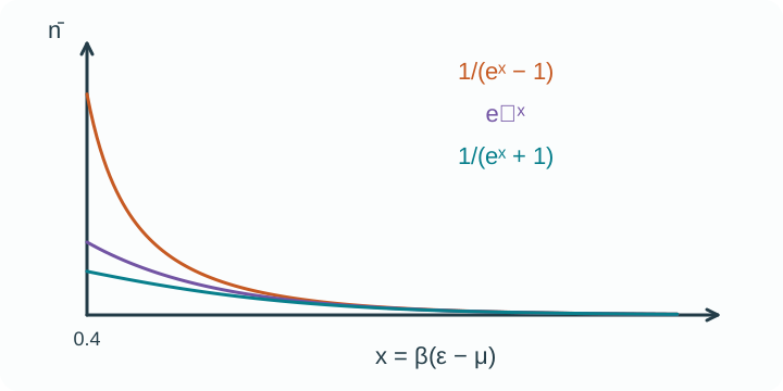
Three decreasing mean occupations for positive x: Bose–Einstein above Maxwell–Boltzmann above Fermi–Dirac. — Here $x = (ε - μ) / (k_{B} T) > 0$ and occupation is per one-particle state, without a density-of-states factor. For large x all three approach the classical result. The Bose occupation can exceed one and diverges as x approaches zero from above; a condensate ground state requires separate treatment. The curves describe an ideal gas in thermal equilibrium.

Bose–Einstein: $\overset{n}{ˉ} = 1/ (exp x - 1)$ , the upper curve.

Maxwell–Boltzmann: $\overset{n}{ˉ} = exp (- x)$ , the middle curve.

Fermi–Dirac: $\overset{n}{ˉ} = 1/ (exp x + 1)$ , the lower curve. The plot covers only $ε > μ$ , not the filled Fermi sea.

Open full-size figure

9.5.1 Grand ensemble → BE/FD distributions

Put noninteracting identical particles in the grand canonical ensemble at $(T, V, μ)$ . With fugacity $z \equiv e^{β μ}$ and one–particle levels ${ϵ_{α}}$ ,

ln Ξ = \mp α \sum ln (1 \mp z e^{- β ϵ_{α}})

upper sign for bosons, lower for fermions. Occupations are

⟨ n_{α} ⟩ = \frac{1}{z ^{- 1} e ^{β ϵ_{α}} \mp 1}

The minus in the denominator gives Bose–Einstein bunching, the plus gives Fermi–Dirac blocking.

9.5.2 Density of states in 3D and continuum replacement

For spin degeneracy $g$ and nonrelativistic dispersion $ϵ = p^{2} /2 m$ in volume $V$ ,

g (ϵ) d ϵ = g \frac{V}{4 π ^{2}} (\frac{2 m}{ℏ ^{2}})^{3/2} ϵ d ϵ

Sums become integrals $\sum_{α} \to \int d ϵ g (ϵ)$ .

Define the thermal wavelength

λ_{T} \equiv \frac{2 π ℏ ^{2}}{m k _{B} T}

and the polylogarithm $Li_{s} (x) \equiv \sum_{k \geq 1} x^{k} / k^{s}$ .

9.5.3 Polylog thermodynamics: N, U, and p

For both bosons and fermions, results compactify via polylogs. Let

g_{s} (z) \equiv Li_{s} (z), f_{s} (z) \equiv - Li_{s} (- z)

Then in $d = 3$ for a uniform nonrelativistic gas,

Bosons $(BE)$

N = \frac{g V}{λ _{T}^{3}} g_{3/2} (z), p = \frac{g k _{B} T}{λ _{T}^{3}} g_{5/2} (z), U = \frac{3}{2} p V

Fermions $(FD)$

N = \frac{g V}{λ _{T}^{3}} f_{3/2} (z), p = \frac{g k _{B} T}{λ _{T}^{3}} f_{5/2} (z), U = \frac{3}{2} p V

The virial identity $U = \frac{3}{2} p V$ holds for any ideal nonrelativistic gas with quadratic dispersion.

9.5.4 Classical limit and the first quantum correction

When $z ≪ 1$ (high $T$ or low $n$ ), both stats reduce to MB since $g_{s} (z) \approx z$ and $f_{s} (z) \approx z$ . Expanding further gives the leading quantum correction to the ideal–gas law

\frac{p}{n k _{B} T} = 1 \pm \frac{1}{2 ^{5/2}} \frac{n λ _{T}^{3}}{g} + O ((n λ_{T}^{3} / g)^{2})

upper sign for fermions (Pauli “repulsion” raises pressure), lower sign for bosons (Bose “attraction” lowers it)

9.5.5 Chemical potential behavior

Bosons: $μ \leq 0$ . At fixed $n$ as $T$ decreases, $μ$ rises toward $0^{-}$ . For an ideal uniform gas, the excited-state capacity is capped by $g_{3/2} (1) = ζ (3/2)$ , leading to Bose–Einstein condensation when $n λ_{T}^{3}$ exceeds a constant. We detail BEC in §9.7.
Fermions: $μ$ is positive at low $T$ and approaches the Fermi energy $ϵ_{F}$ as $T \to 0$ . With $n \equiv N / V$ and spin degeneracy $g$ ,

ϵ_{F} = \frac{ℏ ^{2}}{2 m} (\frac{6 π ^{2} n}{g})^{2/3}, k_{B} T_{F} \equiv ϵ_{F}

At finite but small $T / T_{F}$ , $μ (T)$ decreases from $ϵ_{F}$ by $\sim (T / T_{F})^{2}$ .

9.5.6 Degenerate Fermi gas and the Sommerfeld expansion

For $T ≪ T_{F}$ , evaluate Fermi integrals asymptotically. Let $x \equiv T / T_{F} ≪ 1$ .

Chemical potential

μ (T) = ϵ_{F} [1 - \frac{π ^{2}}{12} x^{2} - \frac{π ^{4}}{80} x^{4} + \dots]

Internal energy and pressure at low $T$

U = \frac{3}{5} N ϵ_{F} [1 + \frac{5 π ^{2}}{12} x^{2} + \dots], p = \frac{2}{5} n ϵ_{F} [1 + \frac{5 π ^{2}}{12} x^{2} + \dots]

Heat capacity per particle

\frac{C _{V}}{N k _{B}} = \frac{π ^{2}}{2} x + O (x^{3})

Linear in $T$ is the signature of a Fermi surface with a thin shell of thermally active states of thickness $\sim k_{B} T$ .

9.5.7 Nondegenerate Bose gas and the edge of BEC

Above condensation (no macroscopic ground-state occupation), $μ < 0$ solves $n λ_{T}^{3} = g g_{3/2} (z)$ . Thermodynamics follows from §9.5.3 with $z < 1$ . As $T$ is lowered at fixed $n$ , $z \to 1^{-}$ , $g_{s} (z) \to ζ (s)$ , and the excited-state density saturates at

n_{ex,max} = \frac{g}{λ _{T}^{3}} ζ (3/2)

The “excess” particles must go into the ground state at and below the critical temperature found in §9.7.

9.5.8 Relativistic and massless limits (teaser)

For massless particles with $ϵ = p c$ , the density of states is $g (ϵ) \propto ϵ^{2}$ . The massive dispersion $ϵ = p^{2} c^{2} + m^{2} c^{4}$ approaches this form only in the ultrarelativistic limit. Massless bosons (photons) have $U \propto V T^{4}$ with $p = U /3 V$ . We develop photons and phonons in §9.6.

9.5.9 Worked mini-examples

(a) Classical limit check

Show that taking $z ≪ 1$ in $N = g V λ_{T}^{- 3} g_{3/2} (z)$ and $p = g k_{B} T λ_{T}^{- 3} g_{5/2} (z)$ reproduces $p V = N k_{B} T$ to leading order and yields the $\pm 2^{- 5/2} n λ_{T}^{3} / g$ correction next.

(b) 3D density of states

Derive $g (ϵ)$ by counting momentum states in a box and using $ϵ = p^{2} /2 m$ .

(c) Fermi energy numerics

For electrons in a metal with $n \approx 8.5 \times 1 0^{28} m^{- 3}$ and $g = 2$ , compute $ϵ_{F}$ and $T_{F}$ , then estimate $C_{V} / (N k_{B})$ at $T = 300 K$ .

(d) Low- $T$ $μ (T)$ for fermions

Use the Sommerfeld expansion of $\int d ϵ ϵ^{1/2} / (e^{β (ϵ - μ)} + 1)$ to obtain the $μ (T)$ series up to $O (x^{4})$ .

(e) Bose gas near $z \to 1^{-}$

Evaluate $g_{3/2} (z)$ numerically close to $z = 1$ using the polylog expansion and show how $n λ_{T}^{3}$ approaches $g ζ (3/2)$ .

9.5.10 Minimal problem kit

Starting from $ln Ξ$ , derive $⟨ n_{α} ⟩$ and the BE/FD forms
Replace sums by $\int d ϵ g (ϵ)$ to obtain the polylog formulas for $N$ , $p$ , and $U$ in $d = 3$
Expand $p / (n k_{B} T)$ in powers of $n λ_{T}^{3}$ and identify the second virial coefficient sign for bosons vs fermions
Derive the Fermi energy $ϵ_{F}$ and $p (T = 0) = \frac{2}{5} n ϵ_{F}$ , then use Sommerfeld to obtain $C_{V} \propto T$
At fixed $n$ for an ideal Bose gas, show $μ \to 0^{-}$ as $T ↓ T_{c}$ and compute the slope $d μ / d T$ at $z ≲ 1$ from the number equation

9.6 Photons & Phonons: Blackbody Radiation and Heat Capacity of Solids

Two archetypal Bose gases, two very different worlds. Photons: massless, spin-1, number not conserved, $μ = 0$ , pressure $p = U /3 V$ , the $T^{4}$ law. Phonons: lattice vibrations with linear dispersion at long wavelengths, three polarizations, and a Debye cutoff that enforces $3 N$ modes. Together they explain the spectrum of light and why solids’ specific heats crash to zero at low $T$ .

9.6.1 Photon gas basics

Photons are created/annihilated freely in thermal equilibrium, so the chemical potential must be zero. Put EM waves in a large cubic cavity of volume $V$ with periodic boundary conditions. Counting transverse modes per angular frequency $ω$ gives the density of states

g (ω) d ω = \frac{V}{π ^{2} c ^{3}} ω^{2} d ω

Bose occupation with $μ = 0$ is $n_{B} (ω) = (e^{β ℏ ω} - 1)^{- 1}$ , yielding the Planck energy density

u (ω) d ω \equiv \frac{d U}{V} = \frac{ℏ ω ^{3}}{π ^{2} c ^{3}} \frac{d ω}{e ^{β ℏ ω} - 1}

The number spectrum follows by dividing by $ℏ ω$

n (ω) d ω = \frac{ω ^{2}}{π ^{2} c ^{3}} \frac{d ω}{e ^{β ℏ ω} - 1}

9.6.2 Stefan–Boltzmann and Wien: two famous corollaries

Integrating $u (ω)$ over all $ω$ gives

\frac{U}{V} \equiv a T^{4}, a = \frac{π ^{2} k _{B}^{4}}{15 ℏ ^{3} c ^{3}}

Radiation pressure for an isotropic photon gas is

p = \frac{1}{3} \frac{U}{V}

The radiative flux from a black surface is $Φ = σ T^{4}$ with

σ = \frac{a c}{4} = \frac{π ^{2} k _{B}^{4}}{60 ℏ ^{3} c ^{2}}

The wavelength of peak spectral exitance satisfies Wien’s displacement

λ_{max} T = b, b \approx 2.898 \times 1 0^{- 3} m \cdot K

obtained by maximizing the $λ$ -form of Planck’s law.

Entropy density and enthalpy follow from $p = U /3 V$ :

s \equiv \frac{S}{V} = \frac{4}{3} a T^{3}, h \equiv \frac{U + p V}{V} = \frac{4}{3} a T^{4}

9.6.3 Phonons: quantized sound with linear dispersion

In a crystal, small lattice displacements form normal modes. At long wavelengths the acoustic branches have

ω = v_{s} k

with sound speed $v_{s}$ and three polarizations (one longitudinal, two transverse). Treating them as a gas of noninteracting bosons, the Bose occupation is the same $n_{B} (ω)$ , but the density of states uses $v_{s}$ instead of $c$ and must be cut off to enforce a finite number of modes.

Debye’s key move: approximate the acoustic branches as linear up to a cutoff $k_{D}$ chosen so that the total number of modes equals $3 N$ for $N$ atoms

\frac{V}{2 π ^{2}} \int_{0}^{k_{D}} k^{2} d k \times 3 = 3 N \Rightarrow k_{D} = (6 π^{2} \frac{N}{V})^{1/3}

Define the Debye frequency and Debye temperature

ω_{D} \equiv v_{s} k_{D}, Θ_{D} \equiv \frac{ℏ ω _{D}}{k _{B}}

A single “average” $v_{s}$ captures the three polarizations to good accuracy for bulk thermodynamics.

9.6.4 Debye model

The phonon internal energy omitting zero-point pieces is

U = \int_{0}^{ω_{D}} d ω g_{D} (ω) ℏ ω n_{B} (ω)

with Debye density of states

g_{D} (ω) = \frac{9 N}{ω _{D}^{3}} ω^{2}

Change variables $x \equiv ℏ ω / k_{B} T$ to obtain the standard Debye heat capacity

C_{V} = 9 N k_{B} (\frac{T}{Θ _{D}})^{3} \int_{0}^{Θ_{D} / T} d x \frac{x ^{4} e ^{x}}{( e ^{x} - 1 ) ^{2}}

Asymptotics:

Low $T$ $(T ≪ Θ_{D})$

C_{V} ≃ \frac{12 π ^{4}}{5} N k_{B} (\frac{T}{Θ _{D}})^{3}

High $T$ $(T ≫ Θ_{D})$

C_{V} \to 3 N k_{B}

recovering Dulong–Petit.

9.6.5 Einstein model: optical modes and the crossover

Einstein imagined each atom as an independent oscillator of a single frequency $ω_{E}$ . Then

C_{V}^{Ein} = 3 N k_{B} \frac{x ^{2} e ^{x}}{( e ^{x} - 1 ) ^{2}}, x \equiv \frac{ℏ ω _{E}}{k _{B} T}

It captures the high- $T$ limit and the exponential freeze-out at low $T$ , but misses the $T^{3}$ law because it lacks low-frequency acoustic modes. Real crystals often interpolate: optical modes look Einstein-like, acoustic modes look Debye-like.

9.6.6 Phonon gas thermodynamics

With $ω = v_{s} k$ and three polarizations, the energy density of a free phonon gas at low $T ≪ Θ_{D}$ mirrors photons with $c \to v_{s}$ and a factor $3/2$ because three acoustic branches replace two photon polarizations

u_{ph} (T) \propto \frac{( k _{B} T ) ^{4}}{ℏ ^{3} v _{s}^{3}}

Differentiating gives $C_{V} \propto T^{3}$ as in Debye. In a solid, the “pressure” of phonons modifies the elastic response rather than pushing on a volume like a gas, but the scaling intuition is identical.

9.6.7 Blackbodies in nature: quick tour

Cosmic microwave background is a near-perfect blackbody at $T \approx 2.725 K$ , a fossil photon gas filling the universe
Stars approximate blackbodies over parts of their spectrum; deviations encode atmospheres and lines
Laboratory cavities with small apertures mimic blackbody emitters and set radiometry standards

9.6.8 Common pitfalls

Forgetting $μ = 0$ for photons. Any attempt to fix photon number in equilibrium is unphysical unless you also constrain the spectrum with pumping
Mixing $ω$ and $λ$ peaks. The maximum of $u_{ω}$ and of $u_{λ}$ occur at different places; Wien’s $b$ refers to the wavelength peak
Ignoring polarizations or cutoffs. Debye needs $3 N$ modes total; missing the factor 3 or the cutoff breaks $C_{V}$
High- $T$ limit with quantum units. Always check $Θ_{D} / T$ or $x = ℏ ω / k_{B} T$ before claiming “classical” behavior

9.6.9 Worked mini-examples

(a) Recover Stefan–Boltzmann.
Integrate $u (ω)$ using $\int_{0}^{\infty} d x x^{3} / (e^{x} - 1) = π^{4} /15$ after $x = β ℏ ω$ to obtain $U / V = a T^{4}$ and $p = U /3 V$ .

(b) Wien’s displacement.
Maximize the wavelength spectral density to show $λ_{max} T = b$ and extract $b$ numerically from the transcendental equation.

(c) Debye low- $T$ asymptotic.
Expand the Debye integral for $Θ_{D} / T \to \infty$ to derive $C_{V} ≃ (12 π^{4} /5) N k_{B} (T / Θ_{D})^{3}$ .

(d) Einstein vs Debye at intermediate $T$ .
Plot $C_{V} / (3 N k_{B})$ vs $T /Θ$ for both models and explain why real data usually bends between them.

(e) Photon gas entropy density.
Using $p = U /3 V$ and $d U = T d S - p d V$ , derive $s = (4/3) a T^{3}$ .

9.6.10 Minimal problem kit

Starting from the cavity mode count, derive $g (ω)$ and Planck’s $u (ω)$
Prove $p = U /3 V$ by averaging the Maxwell stress tensor for isotropic radiation
Show that the phonon mode count with Debye cutoff equals $3 N$ and obtain $k_{D}$
Evaluate the Debye heat capacity integral numerically for $T / Θ_{D} = {0.05, 0.2, 1, 3}$ and compare to Einstein’s prediction at the same $T$ using $ω_{E} \approx 0.806 ω_{D}$
Derive the $T^{4}$ scaling of the low- $T$ phonon energy density by mapping the photon calculation with $c \to v_{s}$

9.7 Bose–Einstein Condensation & Degenerate Fermi Gas

Turn the dial to low temperature and high phase-space density and quantum statistics starts making executive decisions. Bosons pile into the ground state → Bose–Einstein condensation (BEC). Fermions lock into a Fermi sea with Pauli pressure. We build the ideal-gas baseline for BEC in 3D, add traps and interaction corrections, sketch superfluidity via Bogoliubov, and recap the degenerate Fermi gas with a couple of “why this matters” stops.

9.7.1 BEC in a uniform ideal Bose gas (3D)

From §9.5, for noninteracting bosons

N = \frac{g V}{λ _{T}^{3}} g_{3/2} (z)

with $z = e^{β μ}$ and $g_{s}$ the polylog. Because $g_{3/2} (z) \leq g_{3/2} (1) = ζ (3/2)$ , the excited states can hold at most

N_{ex, max} = \frac{g V}{λ _{T}^{3}} ζ (3/2)

At fixed density $n = N / V$ , lowering $T$ decreases $1/ λ_{T}^{3} \propto T^{3/2}$ and hence the maximum excited-state capacity. The temperature where this capacity equals the total particle number is the critical temperature

T_{c} = \frac{2 π ℏ ^{2}}{m k _{B}} (\frac{n}{g ζ ( 3/2 )})^{2/3}

Below $T_{c}$ , the chemical potential pins to $μ = 0$ and the condensed fraction is

\frac{N _{0}}{N} = 1 - (\frac{T}{T _{c}})^{3/2}

Thermodynamics below $T_{c}$ comes entirely from excitations ( $N_{0}$ contributes no energy in the ideal gas):

p = \frac{g k _{B} T}{λ _{T}^{3}} ζ (5/2), U = \frac{3}{2} p V

Specific heat per particle for $T < T_{c}$

\frac{C _{V}}{N k _{B}} = \frac{15}{4} \frac{ζ ( 5/2 )}{ζ ( 3/2 )} (\frac{T}{T _{c}})^{3/2}

Above $T_{c}$ , $μ < 0$ solves $n λ_{T}^{3} = g g_{3/2} (z)$ and $C_{V}$ approaches the classical $3 N k_{B} /2$ at high $T$ . At $T_{c}$ the ideal-gas $C_{V}$ shows a cusp.

9.7.2 No BEC in uniform 1D/2D at finite $T$

For a homogeneous ideal gas, $N_{ex} \propto g_{d /2} (z)$ in $d$ dimensions. The series diverges at $z \to 1^{-}$ for $d \leq 2$ : in two dimensions $g_{1} (1)$ diverges and $g_{1} (z)$ grows logarithmically, while in one dimension the divergence is stronger. So no true BEC occurs in uniform 1D/2D at finite $T$ in the thermodynamic limit; interactions in 2D can still support superfluidity via a Kosterlitz–Thouless transition, but that is not a macroscopic population of a single $k = 0$ mode.

9.7.3 Trapped Bose gases: harmonic potential

Experiments confine atoms in approximately harmonic traps $V (r) = \frac{1}{2} m (ω_{x}^{2} x^{2} + ω_{y}^{2} y^{2} + ω_{z}^{2} z^{2})$ . The single-particle density of states becomes $g (ϵ) \propto ϵ^{2} / (ℏ \overset{ω}{ˉ})^{3}$ with geometric mean $\overset{ω}{ˉ} \equiv (ω_{x} ω_{y} ω_{z})^{1/3}$ . The critical temperature for an ideal trapped gas is

k_{B} T_{c}^{trap} = ℏ \overset{ω}{ˉ} (\frac{N}{ζ ( 3 )})^{1/3}

and, for $T < T_{c}^{trap}$ ,

\frac{N _{0}}{N} = 1 - (\frac{T}{T _{c}^{trap}})^{3}

The steeper exponent reflects the different density of states.

9.7.4 Canonical vs grand-canonical fluctuations: the “catastrophe”

In the grand canonical ensemble for an ideal BEC below $T_{c}$ , a macroscopically occupied ground state has $Var (N_{0}) \sim O (N^{2})$ ; this reservoir-based result is unsuitable for a finite cloud with fixed particle number. The canonical ensemble enforces fixed total $N$ , but the remaining scaling depends on the spectrum. In the usual condensed regime, a three-dimensional harmonic trap gives $Var (N_{0}) \sim O (N)$ , whereas a uniform three-dimensional ideal gas at fixed density has $Var (N_{0}) \sim O (N^{4/3})$ . Choose both the ensemble and the confinement appropriate to the experiment.

9.7.5 Interactions and the Gross–Pitaevskii (GP) mean field

At ultracold $T$ , $s$ -wave scattering dominates with amplitude set by the scattering length $a$ . The effective coupling is

g_{int} = \frac{4 π ℏ ^{2} a}{m}

For a weakly interacting condensate with macroscopic wavefunction $Ψ (r, t)$ ,

i ℏ \partial_{t} Ψ = [- \frac{ℏ ^{2} \nabla ^{2}}{2 m} + V (r) + g_{int} ∣Ψ ∣^{2}] Ψ

This is the Gross–Pitaevskii equation. In uniform matter with density $n = ∣Ψ ∣^{2}$ ,

μ = g_{int} n, c = \frac{g _{int} n}{m}, ξ \equiv \frac{ℏ}{2 m c}

where $c$ is the sound speed and $ξ$ the healing length, the scale over which the order parameter recovers near defects or boundaries.

9.7.6 Bogoliubov spectrum and superfluidity (sketch)

Linearizing fluctuations around the condensate gives the Bogoliubov dispersion

ϵ_{k} = (\frac{ℏ ^{2} k ^{2}}{2 m})^{2} + c^{2} ℏ^{2} k^{2}

Low $k$ is phononic $ϵ_{k} \approx ℏ c k$ and high $k$ crosses over to free-particle $ϵ_{k} \approx ℏ^{2} k^{2} /2 m$ . The Landau criterion sets the critical flow speed

v_{c} = k min \frac{ϵ _{k}}{ℏ k} = c

which is why weakly interacting BECs are superfluids with frictionless flow below $c$ .

9.7.7 Degenerate Fermi gas recap: T=0 and small T

From §9.5, the noninteracting Fermi gas has Fermi energy

ϵ_{F} = \frac{ℏ ^{2}}{2 m} (\frac{6 π ^{2} n}{g})^{2/3}, p (0) = \frac{2}{5} n ϵ_{F}, U (0) = \frac{3}{5} N ϵ_{F}

Finite- $T$ corrections follow from the Sommerfeld expansion: $C_{V} \propto T$ , $μ (T) \approx ϵ_{F} [1 - \frac{π ^{2}}{12} (T / T_{F})^{2} + \dots]$ . The pressure at $T = 0$ embodies Pauli pressure, stabilizing systems from collapse and setting scales in metals and compact objects.

Harmonic trap. For $N$ fermions in a 3D harmonic trap with $\overset{ω}{ˉ}$ , the $T = 0$ Fermi energy is

ϵ_{F}^{trap} = ℏ \overset{ω}{ˉ} (6 N / g)^{1/3}

and the cloud radius follows from a Thomas–Fermi profile.

9.7.8 Two quick applications

White dwarfs (cartoon). Electrons form a highly degenerate gas. In the relativistic limit, $p \sim n^{4/3}$ instead of $n^{5/3}$ , which leads to a maximum supported mass (Chandrasekhar limit). The point is qualitative here: degeneracy pressure is real, thermal pressure is optional.
Cold-atom labs. Feshbach resonances tune $a$ across zero → weakly interacting BECs, strongly interacting unitary Fermi gases, and the BEC–BCS crossover. Bogoliubov sound and collective modes are textbook confirmations of the theory above.

9.7.9 Common pitfalls

Forgetting that $μ = 0$ below $T_{c}$ for the ideal Bose gas. Don’t force a negative $μ$ once the condensate forms
Using grand-canonical fluctuations for a fixed- $N$ trap. Canonical variance is the right one for cold-atom clouds
Claiming uniform 2D BEC. Not at finite $T$ ; look for KT superfluidity instead
Treating interactions as “small” without checking $n a^{3}$ . Weak-coupling GP/Bogoliubov needs $n a^{3} ≪ 1$

9.7.10 Worked mini-examples

(a) $T_{c}$ for a typical BEC.
Take $^{87} Rb$ with $m \approx 1.44 \times 1 0^{- 25} kg$ , $g = 1$ , and density $n = 1 0^{20} m^{- 3}$ . Plug into the $T_{c}$ formula and estimate the condensate fraction at $T = 0.5 T_{c}$ .

(b) No BEC in 2D.
Show $N_{ex} \propto g_{1} (z)$ diverges as $z \to 1^{-}$ for a uniform 2D gas by converting the sum to an integral and identifying the logarithm.

(c) Trap $T_{c}$ .
Given $N = 2 \times 1 0^{5}$ atoms and $\overset{ω}{ˉ} = 2 π \times 100 Hz$ , compute $T_{c}^{trap}$ and the condensed fraction at $0.7 T_{c}^{trap}$ .

(d) Healing length.
For $a = 5 nm$ and $n = 1 0^{20} m^{- 3}$ , estimate $g_{int}$ , $c$ , and $ξ$ .

(e) Bogoliubov slope.
Verify that $ϵ_{k} \approx ℏ c k$ at $k ≪ 1/ ξ$ and find the crossover $k$ where the dispersion deviates by, say, $10%$ .

(f) Fermi pressure number check.
For electrons with $n = 8 \times 1 0^{28} m^{- 3}$ , compute $ϵ_{F}$ and $p (0) = \frac{2}{5} n ϵ_{F}$ ; compare to atmospheric pressure.

9.7.11 Minimal problem kit

Derive $T_{c}$ and the condensed fraction for a uniform ideal Bose gas, then repeat for a harmonic trap using the appropriate density of states
Starting from $p = (g k_{B} T / λ_{T}^{3}) ζ (5/2)$ , compute $C_{V}$ below $T_{c}$ and show the cusp at $T_{c}$
Show explicitly why $g_{3/2} (1)$ converges in 3D but $g_{1} (1)$ diverges in 2D, and relate this to the absence of uniform 2D BEC
Linearize the GP equation around a uniform solution and derive the Bogoliubov dispersion and Landau critical velocity
Use the Sommerfeld expansion to obtain $U (T)$ and $C_{V} (T)$ of a 3D Fermi gas through order $(T / T_{F})^{2}$ ; derive $ϵ_{F}^{trap}$ for a harmonic confinement

9.8 Mean-Field & Landau Theory: Order Parameters, van der Waals, Curie–Weiss

Mean-field is the “group project” approximation: every degree of freedom feels the average of everyone else. It often nails the shape of phase diagrams and gives analytic critical exponents. Landau theory turns that idea into a controlled expansion in the order parameter and symmetries. This section builds Curie–Weiss magnetism, the van der Waals fluid with Maxwell construction, Landau free energies and exponents, correlation length from Landau–Ginzburg, the Ginzburg criterion, and where first-order and tricritical points sneak in.

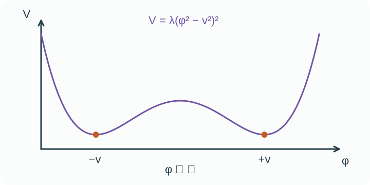
For a real scalar order parameter, an even double well has two symmetry related minima. Choosing either minimum breaks the reflection symmetry.

9.8.1 What mean-field assumes

Pick an order parameter $ϕ$ that flips sign under the broken symmetry:

Ferromagnet: $ϕ \equiv m$ (magnetization density), symmetry $m \to - m$
Liquid–gas: $ϕ \equiv n - n_{c}$ (density deviation), no Ising symmetry but same math near $T_{c}$

Mean-field idea: Replace neighbors by their average. Fluctuations are ignored when coordination is high or the interaction is long-ranged, which gets increasingly true in higher spatial dimension $d$ .

9.8.2 Curie–Weiss ferromagnet (Ising-like, z neighbors)

Start with Ising spins $σ_{i} = \pm 1$ , coupling $J > 0$ , field $h$ . In mean-field each spin sees an effective field $h_{eff} = h + z J m$ with $m \equiv ⟨ σ ⟩$ . The single-site partition function is $z_{1} = 2 cosh (β h_{eff})$ , giving the self-consistency equation

m = tanh [β (h + z J m)]

At $h = 0$ , expand for small $m$ to get the Curie–Weiss critical temperature

k_{B} T_{c} = z J

Critical behavior:

$T > T_{c}$ small $h$ : $m \approx χ h$ with

χ = \frac{1}{k _{B} ( T - T _{c} )}

so $γ_{MF} = 1$

$T < T_{c}$ at $h = 0$ : nonzero solutions appear

m \sim (1 - \frac{T}{T _{c}})^{1/2}

so $β_{MF} = 1/2$

At $T = T_{c}$ , $m \propto h^{1/3}$ , so $δ_{MF} = 3$

Specific heat has a finite jump (no divergence): $α_{MF} = 0$

9.8.3 Landau free energy: symmetry dictates the form

Write an analytic expansion in the order parameter consistent with symmetries. For an Ising-like scalar $m$ in a uniform system

F (m; T, h) = F_{0} (T) + a_{2} t m^{2} + a_{4} m^{4} + a_{6} m^{6} - h m

with temperature deviation $t \equiv T - T_{c}$ and $a_{4} > 0$ for a standard second-order transition. Near this ordinary critical point, truncate at quartic order, neglecting the sextic term in the following minimization and leading critical formulas:

\frac{\partial F}{\partial m} = 2 a_{2} t m + 4 a_{4} m^{3} - h = 0

Consequences at $h = 0$ :

For $t > 0$ : minimum at $m = 0$
For $t < 0$ : minima at

m_{⋆} (t) = \pm \frac{- a _{2} t}{2 a _{4}}

so $β_{MF} = 1/2$

Susceptibility above $T_{c}$ from linear response:

χ^{- 1} = \frac{\partial ^{2} F}{\partial m ^{2}}_{m = 0} = 2 a_{2} t

so $χ \propto t^{- 1}$ and $γ_{MF} = 1$

At $t = 0$ with $h \neq = 0$ :

4 a_{4} m^{3} = h \Rightarrow m \propto h^{1/3}

so $δ_{MF} = 3$

Specific heat jump. Plug $m_{⋆}$ into $F$ :

F_{m i n} (t < 0) = F_{0} (T) - \frac{a _{2}^{2}}{4 a _{4}} t^{2}

Therefore $C = - T \partial^{2} F / \partial T^{2}$ gets a finite step at $T_{c}$ , i.e., $α_{MF} = 0$ with a discontinuity.

9.8.4 First order and tricritical

If microscopic physics drives $a_{4} < 0$ , the $m^{4}$ term destabilizes. Stabilize with $a_{6} > 0$ . Then as $t$ varies, two minima at $\pm m$ appear before $t = 0$ and the system jumps at coexistence $t = t_{coex}$ where the wells are equal depth. That jump is a first-order transition with latent heat.

The point where $a_{4}$ changes sign at $t = 0$ is a tricritical point. Landau analysis with $a_{4} = 0$ predicts different exponents, e.g., $m \sim (- t)^{1/4}$ .

9.8.5 Landau–Ginzburg functional and correlation length

Allow slow spatial variations of the order parameter. The Landau–Ginzburg free-energy functional is

F [ϕ] = \int d^{d} r [\frac{r _{0}}{2} ϕ^{2} + \frac{c}{2} (\nabla ϕ)^{2} + \frac{u}{4} ϕ^{4} - h ϕ]

with $r_{0} \propto t$ . In the Gaussian regime ( $u$ small, $t > 0$ ), the two-point correlator in Fourier space has Ornstein–Zernike form

S (k) \equiv ⟨ ∣ ϕ_{k} ∣^{2} ⟩ \propto \frac{1}{r _{0} + c k ^{2}}

Define the correlation length

ξ^{2} = \frac{c}{r _{0}} \propto t^{- 1}

hence $ν_{MF} = 1/2$ . In three dimensions the real-space correlator has the form $e^{- r / ξ} / r^{d - 2}$ ; this exponential prefactor is not the general-dimensional formula. At criticality in dimensions greater than two, the Gaussian correlator has the inverse-distance power set by dimension minus two, giving $η_{MF} = 0$ .

9.8.6 Ginzburg criterion: when mean-field breaks

Mean-field ignores order-parameter fluctuations. Compare fluctuation size in a correlation volume $ξ^{d}$ to $m_{⋆}^{2}$ . Roughly,

\frac{⟨ δ ϕ ^{2} ⟩ _{ξ}}{m _{⋆}^{2}} \sim \frac{k _{B} T}{u ξ ^{d} m _{⋆}^{4}}

Using $m_{⋆}^{2} \sim ∣ t ∣/ u$ and $ξ \sim t^{- 1/2}$ gives a Ginzburg number $Gi$ such that mean-field is valid only for

∣ t ∣ ≫ Gi

In short: for $d > 4$ the fluctuation integral is benign and mean-field is asymptotically exact. For $d \leq 4$ , a window close to $T_{c}$ is fluctuation dominated and requires RG (§9.10).

9.8.7 van der Waals fluid: mean-field liquid–gas

Write the equation of state in number-density form $n = N / V$ :

p (n, T) = \frac{n k _{B} T}{1 - bn} - a n^{2}

with excluded-volume $b$ and attraction $a$ . The critical point satisfies $(\partial p / \partial n)_{T_{c}} = (\partial^{2} p / \partial n^{2})_{T_{c}} = 0$ , giving

n_{c} = \frac{1}{3 b}, k_{B} T_{c} = \frac{8 a}{27 b}, p_{c} = \frac{a}{27 b ^{2}}

In molar form $p = RT / (V_{m} - b) - a / V_{m}^{2}$ one gets $V_{c} = 3 b$ , $T_{c} = 8 a / (27 b R)$ , $p_{c} = a / (27 b^{2})$ .

Define reduced variables $p_{r} \equiv p / p_{c}$ , $v_{r} \equiv V_{m} / V_{c}$ , $T_{r} \equiv T / T_{c}$ to get the law of corresponding states

p_{r} = \frac{8 T _{r}}{3 v _{r} - 1} - \frac{3}{v _{r}^{2}}

Below $T_{c}$ , $p (V)$ has an S-shape. The mechanical instability region satisfies $(\partial p / \partial V)_{T} > 0$ ; the spinodals solve $(\partial p / \partial V)_{T} = 0$ . The coexistence pressure at a given $T < T_{c}$ is set by the Maxwell equal-area rule (since $g = μ$ must be equal in both phases).

Near $T_{c}$ the density difference obeys the mean-field law

Δ n \propto (T_{c} - T)^{1/2}

matching $β_{MF} = 1/2$ .

9.8.8 Metastability, nucleation, and spinodals

Landau’s double-well for $t < 0$ with a small field $h$ shows two minima of unequal depth: the higher is metastable. Decay proceeds by nucleation of critical droplets, not captured by static mean-field but hinted by the barrier between minima. Approaching a spinodal the barrier vanishes; susceptibility and correlation length blow up along that limit in mean-field.

9.8.9 Cheat sheet: mean-field exponents and scaling relations

Mean-field exponents (Ising-like):

Exponent	Meaning	Value
$α$	$C \sim ∣ t ∣^{- α}$	$0$ with jump
$β$	$m \sim (- t)^{β}$	$1/2$
$γ$	$χ \sim ∣ t ∣^{- γ}$	$1$
$δ$	$m \sim h^{1/ δ}$ at $t = 0$	$3$
$ν$	$ξ \sim ∣ t ∣^{- ν}$	$1/2$
$η$	$G (r) \sim r^{- (d - 2 + η)}$ at $t = 0$	$0$

Scaling relations (satisfied by MF):

Widom: $γ = β (δ - 1)$
Rushbrooke: $α + 2 β + γ = 2$
Josephson (hyperscaling): $2 - α = d ν$
- With mean-field exponents it holds at $d = d_{c} = 4$ at the level of power laws (logarithmic corrections may occur); it fails for $d > d_{c}$ . Below $d_{c}$ , use the fluctuation-corrected exponents.

9.8.10 Common pitfalls

Forcing $m \neq = 0$ above $T_{c}$ at $h = 0$ . In Landau with $a_{4} > 0$ , the only minimum for $t > 0$ is $m = 0$
Confusing coexistence with spinodal. Maxwell construction sets coexistence; spinodal is the limit of metastability where $(\partial p / \partial V)_{T} = 0$
Ignoring symmetry. If the symmetry forbids odd terms, don’t insert them by hand. If a field $h$ breaks it, include $- hm$
Declaring MF “exact”. Good far from $T_{c}$ , in high $d$ , or with long-range interactions; close to $T_{c}$ in $d \leq 4$ see §9.10

9.8.11 Worked mini-examples

(a) Curie–Weiss $χ$
Linearize $m = tanh [β (z J m + h)]$ for small $m$ at $h = 0$ to derive $χ = 1/ [k_{B} (T - T_{c})]$ and identify $T_{c}$ .

(b) Landau $m (T)$ and $C$ -jump
Minimize $F = a_{2} t m^{2} + a_{4} m^{4}$ at $h = 0$ for $t < 0$ to get $m_{⋆}^{2} = - a_{2} t / (2 a_{4})$ . Insert into $F$ and compute the specific-heat discontinuity at $T_{c}$ .

(c) Ornstein–Zernike
From the quadratic LG functional, derive $S (k) \propto 1/ (r_{0} + c k^{2})$ and identify $ξ = c / r_{0}$ .

(d) van der Waals critical point
Using $p = n k_{B} T / (1 - bn) - a n^{2}$ , set $\partial_{n} p = \partial_{n}^{2} p = 0$ to find $(n_{c}, T_{c}, p_{c})$ ; then write the reduced EOS.

(e) Tricritical scaling
Set $a_{4} = 0$ , keep $a_{6} > 0$ , minimize $F = a_{2} t m^{2} + a_{6} m^{6}$ . Show $m \sim (- t)^{1/4}$ and extract $β_{tri}$ .

9.8.12 Minimal problem kit

Derive the MF exponents $α, β, γ, δ$ from the Landau polynomial and verify Widom and Rushbrooke relations
Starting from the LG functional, compute the real-space correlator $G (r)$ in $d$ dimensions and confirm $η_{MF} = 0$
Apply the Ginzburg criterion to estimate the width $∣ t ∣ ≲ Gi$ of the non-MF critical region for a 3D Ising-like magnet with given $u$ and $c$
For van der Waals, implement the Maxwell equal-area construction analytically near $T_{c}$ and show $Δ n \propto (T_{c} - T)^{1/2}$
Explore the first-order case with $a_{4} < 0$ : find coexistence $t_{coex}$ by equating well depths and locate the spinodals where the second derivative at a minimum vanishes

9.9 The Ising Model: Transfer Matrices, Duality, and Exact 2D Criticality

If statistical physics had a mascot, it’d be the Ising model: spins $σ_{i} = \pm 1$ talking only to neighbors, yet somehow recreating the drama of phase transitions. In 1D it’s chill (no finite- $T$ transition). In 2D it’s iconic: an exact critical point with non-mean-field exponents and logarithmic specific-heat blow-up. This section does the 1D exact solution, domain-wall intuition, Kramers–Wannier duality, Onsager’s highlights, and the scaling data you actually use.

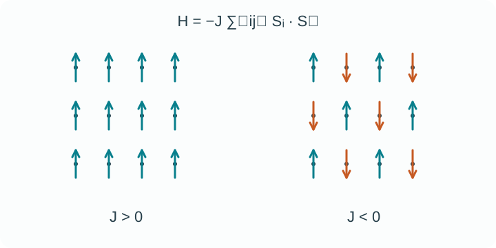
Parallel spins compared with alternating neighboring spins on a bipartite lattice.

9.9.1 Definition and notation

On a lattice with nearest neighbors $⟨ ij ⟩$ and external field $H$ ,

H ({σ}) = - J ⟨ ij ⟩ \sum σ_{i} σ_{j} - H i \sum σ_{i}

We will also use the dimensionless couplings

K \equiv β J, \tilde{h} \equiv β H

Positive $J$ favors alignment (ferromagnet). Partition function $Z = \sum_{{σ}} e^{- β H ({σ})}$ .

9.9.2 1D chain: transfer matrix exact solution

For a ring of $N$ spins (periodic boundary conditions), build the $2 \times 2$ transfer matrix

T_{σ, σ^{'}} = exp [K σ σ^{'} + \frac{h ~}{2} (σ + σ^{'})]

Its eigenvalues are

λ_{\pm} = e^{K} cosh \tilde{h} \pm e^{2 K} sinh^{2} \tilde{h} + e^{- 2 K}

Thermodynamics in the $N \to \infty$ limit is governed by $λ_{+}$ :

f \equiv - \frac{1}{βN} ln Z = - \frac{1}{β} ln λ_{+}

In zero field $\tilde{h} = 0$ ,

λ_{+} = 2 cosh K, λ_{-} = 2 sinh K

There is no spontaneous magnetization at any $T > 0$ , i.e., $m = lim_{\tilde{h} \to 0} \frac{1}{N} \partial_{\tilde{h}} ln Z = 0$ . The connected two-point function decays exponentially,

⟨ σ_{0} σ_{r} ⟩_{c} = (\frac{λ _{-}}{λ _{+}})^{r}

so the correlation length is

ξ^{- 1} = - ln tanh K

Finite at all $T > 0$ , blowing up only at $T = 0$ . Verdict: 1D Ising has no finite- $T$ phase transition.

9.9.3 Domain-wall (kink) intuition: why 1D stays disordered

Flip a contiguous block and you create two domain walls, each costing energy $2 J$ . But their entropy grows like $ln N$ (many places to put them). The free energy of a wall pair is $Δ F \sim 2 \cdot 2 J - k_{B} T ln N$ , so for any $T > 0$ and large $N$ the entropic term wins → domain walls proliferate → long-range order is washed out. In 2D the energy grows with perimeter, and entropy competes differently, allowing a finite $T_{c}$ .

9.9.4 2D square lattice

Kramers–Wannier duality maps the partition function at coupling $K$ to that at a dual coupling $K^{⋆}$ via

sinh (2 K) sinh (2 K^{⋆}) = 1

The critical point sits at self-duality, $K = K^{⋆}$ , giving

sinh (2 K_{c}) = 1

Equivalently,

\frac{k _{B} T _{c}}{J} = \frac{2}{ln ( 1 + 2 )}

For anisotropic couplings $J_{x}, J_{y}$ , the critical line is $sinh (2 K_{x}) sinh (2 K_{y}) = 1$ .

9.9.5 Onsager’s solution: exact critical behavior (at H=0)

The full free energy at $H = 0$ is exactly known (we won’t rewrite the integral here), but the key outputs are:

Specific heat diverges logarithmically

C \sim - ln ∣ t ∣, t \equiv \frac{T - T _{c}}{T _{c}}

so $α = 0$ with a log

Spontaneous magnetization for $T < T_{c}$ (Yang)

m (T) = [1 - sinh^{- 4} (2 K)]^{1/8}

Critical exponents (2D Ising universality)

α = 0, β = \frac{1}{8}, γ = \frac{7}{4}, δ = 15, ν = 1, η = \frac{1}{4}

Correlation length diverges as $ξ \sim ∣ t ∣^{- ν}$ with $ν = 1$ ; the critical correlator decays as $G (r) \sim r^{- d + 2 - η} = r^{- 1/4}$ in 2D

The 2D Ising critical point is also a conformal field theory with central charge $c = \frac{1}{2}$ (useful later for finite-size scaling and exact amplitude ratios).

9.9.6 Transfer matrices, scaling, and finite-size tricks

Transfer-matrix ↔ quantum mapping. The 2D classical Ising model maps to the 1D quantum transverse-field Ising chain via Trotter decomposition. Classical $T = T_{c}$ $\leftrightarrow$ quantum zero-temperature critical point. Many finite-size formulas port directly.
Finite-size scaling. In a box of linear size $L$ , susceptibilities and order parameter moments scale at $T_{c}$ as

χ_{m a x} (L) \propto L^{γ / ν} = L^{7/4}, m (T_{c}, L) \propto L^{- β / ν} = L^{- 1/8}

Binder cumulants and crossing methods are practical ways to locate $T_{c}$ in simulations.

9.9.7 What universality buys you

You never need the lattice-level math again. Any 2D short-range system with a $Z_{2}$ symmetry breaking (liquid–gas along the critical isotherm, uniaxial magnets, binary alloys) shares the same exponents and scaling functions near criticality. Landau mean-field (§9.8) is qualitatively right but its exponents differ; renormalization (§9.10) explains why.

9.9.8 Common pitfalls

Forgetting 1D has no finite- $T$ order. If your code finds $m \neq = 0$ in 1D at $T > 0$ with $H = 0$ , you’re finite-size–fooled or symmetry-broken by the algorithm
Mixing fields. The closed-form $m (T)$ above is only for $H = 0$ ; turning on $H$ destroys the critical singularities in that exact way
Wrong $T_{c}$ . It’s $sinh (2 K_{c}) = 1$ , not $tanh$ or $cosh$ ; equivalently $k_{B} T_{c} / J = 2/ ln (1 + 2)$
Mean-field exponents in 2D. MF gives $β = 1/2$ , $γ = 1$ , etc.—not correct for 2D Ising; use the exact set above
Correlation length sign errors. In 1D, $ξ^{- 1} = - ln (tanh K)$ ; note the minus sign and that $tanh K < 1$ for $T > 0$

9.9.9 Worked mini-examples

(a) 1D transfer matrix at $H = 0$ .
Derive $λ_{\pm} = 2 (cosh K, sinh K)$ , get $f = - k_{B} T ln (2 cosh K)$ , and show $ξ^{- 1} = - ln tanh K$ .

(b) Kramers–Wannier duality.
Starting from high-temperature and low-temperature series for $ln Z$ , show that up to a prefactor they coincide under $sinh (2 K) sinh (2 K^{⋆}) = 1$ , then deduce $K_{c}$ from self-duality.

(c) Magnetization check.
Verify $m (T \to 0) \to 1$ from $m (T) = [1 - sinh^{- 4} (2 K)]^{1/8}$ and that $m (T \to T_{c}^{-}) \sim ∣ t ∣^{1/8}$ .

(d) Finite-size scaling of $χ$ .
Assuming $χ (t, L) = L^{γ / ν} Φ (t L^{1/ ν})$ , show that the peak value scales as $L^{7/4}$ in 2D and how you’d extract $ν$ from data collapse.

(e) 1D domain-wall gas.
Treat kinks as noninteracting with fugacity $y \equiv e^{- 2 K}$ . Show the two-point function $\propto (1 - 2 y)^{r}$ at leading order, reproducing $ξ^{- 1} \approx - ln (1 - 2 y)$ for $y ≪ 1$ .

9.9.10 Minimal problem kit

Build the 1D transfer matrix with field $\tilde{h}$ and derive $λ_{\pm}$ and $f (T, \tilde{h})$ ; compute $m = \partial_{\tilde{h}} ln λ_{+}$ and check $m (\tilde{h} \to 0) = 0$ for $T > 0$
Use duality to get the anisotropic 2D critical line $sinh (2 K_{x}) sinh (2 K_{y}) = 1$ ; reduce to the isotropic $sinh (2 K_{c}) = 1$
From the exact $m (T)$ , extract $β = 1/8$ and confirm the Widom relation $γ = β (δ - 1)$ with $δ = 15$ and $γ = 7/4$
Show that the 2D specific heat behaves as $C \sim - ln ∣ t ∣$ by expanding Onsager’s free-energy integral near $T_{c}$
Map the 2D classical model to the 1D quantum transverse-field Ising chain and identify the quantum critical point in terms of transverse field and exchange

9.10 Critical Phenomena & Renormalization Group Basics

Close to a continuous phase transition the system forgets microscopic details and becomes scale invariant. Correlation length $ξ$ blows up, fluctuations span all sizes, and thermodynamics develops power laws with universal exponents. The renormalization group (RG) turns this into math: coarse-grain, rescale, track how couplings flow. Fixed points rule the neighborhood, and their eigenvalues set the exponents.

9.10.1 Why mean-field breaks

Mean-field pretends fluctuations are small. But at a critical point the correlation length

ξ \sim ∣ t ∣^{- ν}, t \equiv \frac{T - T _{c}}{T _{c}}

diverges, the correlator at $t = 0$ becomes a power law

G (r) \equiv ⟨ ϕ (r) ϕ (0) ⟩_{c} \sim \frac{1}{r ^{d - 2 + η}}

and the free-energy density’s singular part scales like $f_{s} \sim ξ^{- d}$ . You cannot expand around a single length scale when there isn’t one.

9.10.2 Scaling hypothesis and homogeneity laws

Assume the singular free-energy density satisfies a homogeneity relation under rescaling by factor $b > 0$

f_{s} (t, h) = b^{- d} f_{s} (t b^{y_{t}}, h b^{y_{h}})

Here $h$ is the field conjugate to the order parameter. Choose $b = ∣ t ∣^{- 1/ y_{t}}$ and identify exponents:

Specific heat $C \sim - \partial^{2} f_{s} / \partial T^{2} \sim ∣ t ∣^{- α}$ with

2 - α = \frac{d}{y _{t}} \equiv d ν

Order parameter $m \equiv - \partial f_{s} / \partial h ∣_{h \to 0} \sim ∣ t ∣^{β}$ with

β = \frac{d - y _{h}}{y _{t}}

Susceptibility $χ \equiv \partial m / \partial h ∣_{h \to 0} \sim ∣ t ∣^{- γ}$ with

γ = \frac{2 y _{h} - d}{y _{t}}

At $t = 0$ , pick $b = h^{- 1/ y_{h}}$ to get $m \sim h^{1/ δ}$ with

δ = \frac{y _{h}}{d - y _{h}}

Fisher’s relation links $η$ to $y_{h}$ via the critical correlator:

2 - η = 2 y_{h} - d

Collecting the classic scaling relations

Widom: $γ = β (δ - 1)$
Rushbrooke: $α + 2 β + γ = 2$
Josephson (hyperscaling): $2 - α = d ν$
Fisher: $γ = (2 - η) ν$

Hyperscaling typically holds below the upper critical dimension $d_{c}$ .

9.10.3 Kadanoff’s block spin: the cartoon that works

Coarse-grain spins into blocks of size $b$ , average to get a new field $ϕ^{'}$ , and rescale lengths back to the original lattice. Couplings ${K}$ flow to new couplings ${K^{'}}$ . Iterate:

Relevant directions grow under RG ( $K^{'} - K^{⋆} \sim b^{y} (K - K^{⋆})$ with $y > 0$ )
Irrelevant directions shrink ( $y < 0$ )
Marginal need higher-order analysis

Criticality is a flow to a nontrivial fixed point $K^{⋆}$ with at least one relevant direction (temperature). The correlation length exponent is the inverse of the thermal eigenvalue:

ν = \frac{1}{y _{t}}

and the field eigenvalue controls $y_{h}$ and thus $η, β, γ, δ$ via §9.10.2.

9.10.4 Wilson’s momentum-shell RG and beta functions

For a scalar order parameter, the Landau–Ginzburg–Wilson (LGW) functional

F [ϕ] = \int d^{d} x [\frac{1}{2} (\nabla ϕ)^{2} + \frac{r}{2} ϕ^{2} + \frac{u}{4 !} ϕ^{4} - h ϕ]

Coarse-grain by integrating out modes in a momentum shell $Λ/ b < ∣ k ∣ < Λ$ , then rescale $x \to x / b$ and $ϕ \to b^{(d - 2 + η) /2} ϕ$ . The couplings flow with “RG time” $ℓ \equiv ln b$ as shown schematically below; the ellipses include mass-dependent loop terms needed to determine the thermal eigenvalue:

\frac{d r}{d ℓ} = 2 r - c_{1} u + \dots, \frac{d u}{d ℓ} = β (u) = ϵ u - c_{2} u^{2} + \dots

with $ϵ \equiv 4 - d$ . Constants $c_{1}, c_{2}$ depend on conventions; what matters:

For $d < 4$ ( $ϵ > 0$ ) there is a Wilson–Fisher fixed point $u^{⋆} \sim ϵ / c_{2}$ giving non-mean-field exponents
For $d > 4$ ( $ϵ < 0$ ) the Gaussian fixed point $u^{⋆} = 0$ is stable and mean-field exponents hold (with possible logs at $d = 4$ )

For the $O (N)$ model, the $ϵ$ -expansion gives the following one-loop correlation-length exponent and leading two-loop anomalous dimension:

ν = \frac{1}{2} + \frac{N + 2}{4 ( N + 8 )} ϵ + O (ϵ^{2})

η = \frac{( N + 2 )}{2 ( N + 8 ) ^{2}} ϵ^{2} + O (ϵ^{3})

For Ising universality ( $N = 1$ ):

ν = \frac{1}{2} + \frac{1}{12} ϵ + \dots, η = \frac{1}{54} ϵ^{2} + \dots

Plugging $ϵ = 1$ gives rough 3D estimates; higher loops plus resummation refine them.

9.10.5 Upper critical dimension and dangerous irrelevant variables

The $ϕ^{4}$ coupling $u$ is marginal at $d = 4$ and irrelevant for $d > 4$ . Yet for $d > 4$ it can be dangerously irrelevant: it vanishes under RG but still controls the amplitude of $m$ below $T_{c}$ , modifying naive hyperscaling. Consequences:

Mean-field exponents $α = 0, β = 1/2, γ = 1, δ = 3, ν = 1/2, η = 0$ hold for $d \geq d_{c} = 4$
Hyperscaling $2 - α = d ν$ fails for $d > 4$ (free-energy density does not scale as $ξ^{- d}$ without $u$ -dependent rescaling)

Logs at $d = 4$ show up, e.g., $C \sim ∣ ln t ∣^{p}$ .

9.10.6 Finite-size scaling and data collapse

With periodic box size $L$ , RG/homogeneity imply the finite-size scaling (FSS) ansatz for the singular part of the free energy

f_{s} (t, h; L) = L^{- d} F (t L^{1/ ν}, h L^{y_{h}})

Observable templates:

Order parameter: $m (t, h = 0; L) = L^{- β / ν} M (t L^{1/ ν})$
Susceptibility: $χ (t; L) = L^{γ / ν} X (t L^{1/ ν})$
Specific heat: $C (t; L) = L^{α / ν} C (t L^{1/ ν})$ up to additive analytic background

Practical wins: Curves for different $L$ collapse when plotted vs $t L^{1/ ν}$ with vertical multiplication by $L^{β / ν}$ for the order parameter or $L^{- γ / ν}$ for susceptibility, and pseudo-critical temperatures shift as

T_{c} (L) - T_{c} (\infty) \propto L^{- 1/ ν}

9.10.7 Universality classes (quick map)

Ising ( $O (1)$ , $Z_{2}$ symmetry): uniaxial magnets, liquid–gas along the critical isotherm, binary alloys
XY ( $O (2)$ ): superfluid helium, planar spins, thin-film superconductors; in 2D has a Kosterlitz–Thouless transition (essential, not power-law)
Heisenberg ( $O (3)$ ): isotropic magnets
Percolation: geometric connectivity transition with its own exponents
Directed percolation: absorbing-state phase transitions (nonequilibrium)

Same dimension + same symmetries + similar conservation rules → same exponents.

9.10.8 KT interlude (2D XY)

In 2D, vortices unbind at $T_{KT}$ with correlation length

ξ \sim exp (\frac{b}{∣ T - T _{KT} ∣})

No standard power-law exponents; instead there is a universal jump of the superfluid stiffness. This is still RG—just on a different flow diagram with vortex fugacity and stiffness as couplings.

9.10.9 Worked mini-examples

(a) Scaling relations in two lines
Start from $f_{s} (t, h) = b^{- d} f_{s} (t b^{y_{t}}, h b^{y_{h}})$ . Derive $α, β, γ, δ$ and verify Widom and Rushbrooke.

(b) One-loop $ϕ^{4}$ shell RG
Integrate modes in $Λ/ b < k < Λ$ for LGW, rescale, and show schematically $d u / d ℓ = ϵ u - c_{2} u^{2}$ and $d r / d ℓ = 2 r - c_{1} u$ . Identify $u^{⋆}$ . To extract $ν = 1/ y_{t}$ to $O (ϵ)$ , retain the mass-dependent one-loop terms omitted by this schematic flow, shift to the critical surface, and linearize there.

(c) Finite-size shift
Assuming $χ (t, L) = L^{γ / ν} X (t L^{1/ ν})$ , show the susceptibility peak location $t^{*} (L) \propto L^{- 1/ ν}$ .

(d) Data collapse recipe
Given Monte Carlo data for $m (T; L)$ in 2D Ising at $H = 0$ , rescale $m \to L^{β / ν} m$ and $T \to (T - T_{c}) L^{1/ ν}$ with $β = 1/8$ , $ν = 1$ . Explain the adjustable parameters and quality checks.

(e) Dangerous irrelevant $u$ above $d_{c}$
In $d > 4$ , show that $m \propto (- t)^{1/2} u^{- 1/2}$ at mean-field level, illustrating how an “irrelevant” coupling sets amplitudes and breaks naive hyperscaling.

9.10.10 Common pitfalls

Using hyperscaling where it fails. Above $d_{c} = 4$ for Ising-like systems, $2 - α = d ν$ is not valid without caveats
Confusing crossover with criticality. A flow near but not at a fixed point shows effective exponents that drift with scale
Ignoring analytic backgrounds. Specific heat often has a non-singular part that can mask small $α$
Forgetting boundary conditions in FSS. Exponents are universal; scaling functions and subleading corrections are not
Mixing KT with power-law scaling. In 2D XY, expect essential singularities and a stiffness jump, not $β, γ$ etc.

9.10.11 Minimal problem kit

From the homogeneity hypothesis, derive the four standard scaling relations and identify the independent exponent set
Compute $ν$ and $η$ to $O (ϵ)$ for the $O (N)$ model and specialize to $N = 1, 2, 3$
Show that at $d = 4$ the Gaussian fixed point is marginal and derive a logarithmic correction to $C$ in $ϕ^{4}$ theory
Use FSS to estimate $ν$ from synthetic or simulated Ising susceptibility peaks at sizes $L = {16, 32, 64, 128}$
For the KT RG flow, write the lowest-order equations for stiffness $K$ and vortex fugacity $y$ , and show the separatrix corresponding to $T_{KT}$

9.11 Linear Response & Fluctuation–Dissipation

Kick a system gently, watch it wiggle. Linear response theory turns small perturbations into universal formulas linking dissipation to equilibrium fluctuations. The retarded correlator sets the response, causality gives Kramers–Kronig, and the fluctuation–dissipation theorem (FDT) glues noise spectra to the imaginary part of susceptibilities. Transport coefficients then drop out from time integrals of current autocorrelations (Green–Kubo).

9.11.1 Setup: source, observable, and response kernel

Perturb an equilibrium Hamiltonian by a weak time-dependent field $h (t)$ coupled to an operator $A$ :

H^{'} (t) = - h (t) A

Measure another observable $B$ . To linear order,

δ ⟨ B (t)⟩ = \int_{- \infty}^{\infty} d t^{'} χ_{B A} (t - t^{'}) h (t^{'})

with causal susceptibility $χ_{B A} (t < 0) = 0$ . In frequency space,

δ ⟨ B (ω)⟩ = χ_{B A} (ω) h (ω)

The power absorbed by a sinusoidal drive $h (t) = h_{0} cos ω t$ is set by the dissipative part $χ_{AA}^{''} (ω)$ .

9.11.2 Kubo formula: quantum and classical limits

In the Heisenberg picture with equilibrium average $⟨ \dots ⟩$ , the retarded susceptibility is

χ_{B A} (t) = \frac{i}{ℏ} Θ (t) ⟨ [B (t), A (0)] ⟩

Equivalently,

χ_{B A} (ω) = \int_{0}^{\infty} d t e^{iω t} \frac{i}{ℏ} ⟨ [B (t), A (0)] ⟩

Classical limit. Replace commutators by $i ℏ$ times Poisson brackets and obtain

χ_{B A} (t) = - Θ (t) β \frac{d}{d t} C_{B A} (t), C_{B A} (t) \equiv ⟨ δ B (t) δ A (0)⟩

This is the time-domain FDT form for conjugate variables.

9.11.3 Causality ⇒ Kramers–Kronig

Causality makes $χ_{B A} (ω)$ analytic in the upper half-plane. Real and imaginary parts are Hilbert transforms:

Re χ (ω) = \frac{1}{π} P \int_{- \infty}^{\infty} d ω^{'} \frac{χ ^{''} ( ω ^{'} )}{ω ^{'} - ω}

χ^{''} (ω) = - \frac{1}{π} P \int_{- \infty}^{\infty} d ω^{'} \frac{Re χ ( ω ^{'} )}{ω ^{'} - ω}

Dissipation $\Leftrightarrow$ dispersion: you cannot have one without the other.

9.11.4 Fluctuation–dissipation theorem in frequency space

Define the symmetrized equilibrium spectral density of $A$ ,

S_{AA} (ω) \equiv \int_{- \infty}^{\infty} d t e^{iω t} \frac{1}{2} ⟨{δ A (t), δ A (0)}⟩

Then the quantum FDT states

S_{AA} (ω) = ℏ coth (\frac{β ℏ ω}{2}) χ_{AA}^{''} (ω)

Classical limit $β ℏ ω ≪ 1$ gives

S_{AA} (ω) = \frac{2 k _{B} T}{ω} χ_{AA}^{''} (ω)

Interpretation: the same modes that dissipate energy when driven also fluctuate at equilibrium, and the ratio is fixed by $T$ (or by $ℏ ω$ at high frequency).

9.11.5 Green–Kubo relations: transport from autocorrelations

Transport coefficients are time integrals of current autocorrelations.

Self-diffusion in $d$ dimensions with velocity $v$ :

D = \frac{1}{d} \int_{0}^{\infty} d t ⟨ v (t) \cdot v (0)⟩

Electrical conductivity for total current $J_{x}$ in volume $V$ :

σ = \frac{β}{V} \int_{0}^{\infty} d t ⟨ J_{x} (t) J_{x} (0)⟩

Shear viscosity from the volume-integrated microscopic stress component $σ_{x y}$ :

η = \frac{β}{V} \int_{0}^{\infty} d t ⟨ σ_{x y} (t) σ_{x y} (0)⟩

Thermal conductivity in an isotropic $d$ -dimensional system, with total heat current $J_{Q}$ (the volume integral of the heat-flux density):

κ = \frac{k _{B} β ^{2}}{d V} \int_{0}^{\infty} d t ⟨ J_{Q} (t) \cdot J_{Q} (0)⟩

All are equilibrium averages with the unperturbed dynamics.

9.11.6 Langevin, Fokker–Planck, and Einstein relation

For a Brownian particle of position $x$ in a viscous fluid,

m \overset{v}{˙} = - γ v + ξ (t)

with Gaussian white noise $⟨ ξ (t) ξ (0)⟩ = 2 γ k_{B} T δ (t)$ . Solving gives the Einstein relation

D = \frac{k _{B} T}{γ}

and velocity autocorrelation $⟨ v (t) v (0)⟩ = (k_{B} T / m) e^{- t / τ}$ with $τ = m / γ$ . The associated Fokker–Planck equation evolves the probability density and relaxes to the Maxwell–Boltzmann steady state.

9.11.7 Noise examples: Johnson–Nyquist and friends

For a resistor $R$ in the classical regime $ℏ ω ≪ k_{B} T$ , the one-sided (positive-frequency) voltage noise spectral density is twice the two-sided density defined in 9.11.4:

S_{V}^{(1)} (ω) = 4 k_{B} T R

The quantum correction multiplies by $\frac{ℏ ω}{2 k _{B} T} coth (β ℏ ω /2)$ . Current noise follows as $S_{I}^{(1)} (ω) = 4 k_{B} T / R$ for a resistor alone. Same logic underlies magnetic noise in NMR, force noise in AFM, and shot-noise limits in mesoscopic conductors.

9.11.8 Onsager reciprocity and microscopic reversibility

When generalized fluxes $J_{i}$ respond to thermodynamic forces $X_{j}$ linearly,

J_{i} = j \sum L_{ij} X_{j}

time-reversal symmetry implies Onsager–Casimir relations

L_{ij} (B) = ϵ_{i} ϵ_{j} L_{ji} (- B)

where $ϵ_{i} = \pm 1$ is the time-reversal parity of $J_{i}$ . At zero magnetic field and for forces/fluxes with the same parity, $L_{ij} = L_{ji}$ . Reciprocity is a macroscopic echo of equilibrium correlation symmetry.

9.11.9 Causality, passivity, and sum rules

Passivity: $χ^{''} (ω) \geq 0$ for $ω > 0$ for stable, passive systems; it encodes positive dissipation.
Sum rules: Moments of $χ^{''} (ω)$ tie to equal-time commutators or static susceptibilities, e.g., an $f$ -sum rule for charge response.
High-frequency tails: Often fixed by short-time operator algebra; useful for checking numerics or truncated models.

9.11.10 Common pitfalls

Using symmetric instead of retarded correlators in $χ$ . The Kubo $χ$ needs the commutator and $Θ (t)$ .
Forgetting ensemble choice. Green–Kubo averages are taken in the equilibrium ensemble matching conserved quantities.
Abusing classical FDT at high frequency. Use the quantum $coth (β ℏ ω /2)$ factor when $ℏ ω ≳ k_{B} T$ .
Mixing response channels. Coupling $H^{'} = - h A$ means the correct FDT relates $S_{AA}$ to $χ_{AA}^{''}$ , not to some other operator.
Ignoring conservation laws. Currents tied to conserved densities have hydrodynamic long-time tails that can alter naive integral convergence.

9.11.11 Worked mini-examples

(a) Kramers–Kronig from causality
Assume $χ (t) = 0$ for $t < 0$ , Fourier transform, and show the Hilbert-transform relations for $Re χ$ and $χ^{''}$ .

(b) Classical FDT in time domain
With $H^{'} = - h (t) A$ and $B = A$ , prove $χ_{AA} (t) = - Θ (t) β \frac{d}{d t} C_{AA} (t)$ and recover $S_{AA} (ω) = \frac{2 k _{B} T}{ω} χ_{AA}^{''} (ω)$ .

(c) Johnson noise
Take a circuit with a resistor only. Using $I (ω) = V (ω) / R$ and FDT, derive $S_{V}^{(1)} = 4 k_{B} TR$ in the classical band.

(d) Diffusion from velocity correlations
For a single Cartesian velocity component with exponential correlator $⟨ v (t) v (0)⟩ = v_{0}^{2} e^{- t / τ}$ , integrate to get $D = v_{0}^{2} τ$ and compare to $D = k_{B} T / γ$ with $v_{0}^{2} = k_{B} T / m$ and $τ = m / γ$ .

(e) Conductivity Green–Kubo
Show that a uniform electric field couples as $H^{'} = + E_{x} J_{x} t$ in the temporal gauge with vector potential equal to minus electric field times time and derive $σ = (β / V) \int_{0}^{\infty} d t ⟨ J_{x} (t) J_{x} (0)⟩$ .

(f) Onsager reciprocity check
For thermoelectric transport with electric and heat currents, write the $2 \times 2$ $L$ -matrix and argue $L_{12} (B) = L_{21} (- B)$ .

9.11.12 Minimal problem kit

Starting from the Kubo formula, prove the quantum FDT $S_{AA} (ω) = ℏ coth (β ℏ ω /2) χ_{AA}^{''} (ω)$
Derive the Einstein relation $D = μ k_{B} T$ by relating mobility $μ$ to the low-frequency limit of the velocity response
Show that $χ^{''} (ω) \geq 0$ for a passive system by evaluating average absorbed power for a sinusoidal drive
From the continuity equation, connect long-time tails of current correlations to hydrodynamic diffusion and discuss convergence of Green–Kubo integrals
Compute $η$ from a microscopic hard-sphere model via the stress autocorrelation and compare to kinetic-theory scaling

9.12 Kinetic Theory & the Boltzmann Equation

Stat mech taught us what equilibrium looks like. Kinetic theory explains how systems move toward it, and what happens while they’re not there. The star is the Boltzmann equation, a mesoscopic evolution law for the one-particle distribution $f (r, v, t)$ . From it, we’ll derive transport coefficients, connect to hydrodynamics, and see where and why the theory breaks.

9.12.1 From micro to meso: the distribution function

Define $f (r, v, t)$ so that $f d^{3} r d^{3} v$ is the expected number of particles in the phase-space cell. Normalize to $N = \int d^{3} r d^{3} v f$ . Conserved densities are moments of $f$ :

n (r, t) = \int d^{3} v f, u (r, t) = \frac{1}{n} \int d^{3} v v f, ε (r, t) = \int d^{3} v \frac{1}{2} m v^{2} f

Pressure tensor and heat flux are higher moments of the peculiar velocity $c \equiv v - u$ .

9.12.2 The Boltzmann equation and molecular chaos

In external force $F$ ,

\frac{\partial f}{\partial t} + v \cdot \nabla_{r} f + \frac{F}{m} \cdot \nabla_{v} f = C [f]

The collision integral $C [f]$ encodes binary collisions. For short-range interactions and molecular chaos (Stosszahlansatz: pre-collision velocities uncorrelated),

C [f] (r, v) = \int d^{3} v_{2} \int d Ω g σ (g, Ω) [f^{'} f_{2}^{'} - f f_{2}]

with $g = ∣ v - v_{2} ∣$ , differential cross section $σ$ , and $f^{'} = f (r, v^{'}, t)$ the post-collision values determined by energy–momentum conservation.

Collision invariants. For any $ψ (v)$ equal to $1$ , $v$ , or $v^{2}$ ,

\int d^{3} v ψ (v) C [f] = 0

leading to local conservation of mass, momentum, and energy.

9.12.3 Local equilibrium = Maxwell–Boltzmann

$C [f] = 0$ (for all cross sections) iff $f$ is a local Maxwellian,

f_{LE} (r, v, t) = n (r, t) (\frac{m}{2 π k _{B} T ( r , t )})^{3/2} exp [- \frac{m ∣ v - u ( r , t ) ∣ ^{2}}{2 k _{B} T ( r , t )}]

This $f_{LE}$ maximizes local entropy density given $n, u, T$ and is the fixed point of collisions.

9.12.4 The H-theorem: entropy grows

Define Boltzmann’s $H \equiv \int d^{3} r d^{3} v f ln f$ . Using the collision integral,

\frac{d H}{d t} = \int d^{3} r d^{3} v C [f] (1 + ln f) \leq 0

with equality only for $f = f_{LE}$ . Identifying $S = - k_{B} H + const$ gives monotone entropy increase toward local equilibrium. Caveats: relies on molecular chaos and binary, dilute collisions; long-range forces and correlated pre-collisions can spoil the proof.

9.12.5 Hydrodynamics as moment equations

Take moments of Boltzmann and use collision invariants to get the Euler (ideal) or Navier–Stokes–Fourier (dissipative) equations. Let $ρ = mn$ , $p = n k_{B} T$ .

Continuity

\partial_{t} ρ + \nabla \cdot (ρ u) = 0

Momentum

\partial_{t} (ρ u) + \nabla \cdot (ρ u u + p I + Π) = n F

Energy

\partial_{t} ε + \nabla \cdot [(ε + p) u + Π \cdot u + q] = n F \cdot u

$Π$ is the viscous stress, $q$ the heat flux. To close these, expand around $f_{LE}$ .

9.12.6 Chapman–Enskog and transport coefficients

Assume weak gradients (small Knudsen number $K n \equiv ℓ / L$ ) and write $f = f_{LE} + f^{(1)} + \dots$ where $f^{(1)}$ is linear in gradients. Solving Boltzmann at first order gives Newtonian viscosity and Fourier heat law:

Π = - η [\nabla u + (\nabla u)^{T} - \frac{2}{3} (\nabla \cdot u) I] - ζ (\nabla \cdot u) I

q = - κ \nabla T

For hard spheres (mass $m$ , diameter $d$ ) at number density $n$ and temperature $T$ ,

η \sim \frac{5}{16 d ^{2}} \frac{m k _{B} T}{π}, κ \sim \frac{75 k _{B}}{64 d ^{2}} \frac{k _{B} T}{πm}

up to modest Sonine-polynomial correction factors; the bulk viscosity $ζ$ vanishes for monatomic ideal gases.

9.12.7 Relaxation-time and BGK models

Exact collision integrals are painful. The Bhatnagar–Gross–Krook (BGK) model replaces $C [f]$ by a single relaxation rate toward local equilibrium:

C_{BGK} [f] = - \frac{f - f _{LE}}{τ}

Choosing $τ$ to match $η$ reproduces first-order hydrodynamics and fixes $κ$ as a prediction. For a monatomic gas, the single-relaxation-time BGK model has $Pr = 1$ , so it cannot independently fit both coefficients. Such relaxation models are widely used in lattice Boltzmann and semiconductor transport. The simpler relaxation time approximation in solids does the same for electron scattering.

9.12.8 Knudsen number, boundary layers, and breakdowns

Hydro regime $K n ≪ 1$ : Navier–Stokes–Fourier valid.
Transition $K n \sim 0.1$ : slip flows, Knudsen layers near walls; need kinetic boundary conditions.
Ballistic $K n ≳ 1$ : free-molecular flow; Boltzmann without gradient expansions or even collisionless Vlasov dynamics (for long-range forces).
Dense gases: Enskog corrections modify $C [f]$ and transport.
Long-range Coulomb: many small-angle deflections → Landau (Fokker–Planck) collision operator.

9.12.9 Quantum Boltzmann and Pauli/Bose factors

For dilute quantum gases at high enough $T$ that coherence lengths are short, the collision term acquires stimulated/blocked final states:

C_{Q} [f] \propto \int d Γ [f^{'} f_{2}^{'} (1 \pm f) (1 \pm f_{2}) - f f_{2} (1 \pm f^{'}) (1 \pm f_{2}^{'})]

upper sign for bosons, lower for fermions. This is the Uehling–Uhlenbeck modification. At very low $T$ in superfluids, kinetic theory must include collective modes (phonons, Bogoliubov quasiparticles).

9.12.10 Boltzmann transport in solids (electrons and phonons)

In crystals, $f (k, r, t)$ evolves in $k$ -space with band velocity $v_{k} = \nabla_{k} ϵ_{k} /ℏ$ and forces from electric fields and Berry curvature (advanced topic). With a relaxation time $τ (k)$ ,

σ_{xx} = e^{2} \int \frac{d ^{3} k}{( 2 π ) ^{3}} τ (k) v_{x}^{2} (- \frac{\partial f _{0}}{\partial ϵ})

reproduces Drude in free-electron bands, while phonon Boltzmann explains lattice thermal conductivity via three-phonon scattering and boundary limits.

9.12.11 Linear response vs kinetic theory: same game, different screens

Green–Kubo (9.11) says transport = time integrals of autocorrelators. Chapman–Enskog says transport = solutions of Boltzmann to first order in gradients. They agree when both apply. Kinetic theory wins when mean free paths and cross sections are explicit; Green–Kubo wins for interacting liquids where quasiparticles are murky but simulations can measure correlations.

9.12.12 Worked mini-examples

(a) Mean free path and viscosity
For hard spheres at number density $n$ with cross section $σ = π d^{2}$ , show $ℓ ≃ 1/ (2 nσ)$ and estimate $η \sim \frac{1}{3} nm \overset{v}{ˉ} ℓ$ ; compare to the Chapman–Enskog value.

(b) BGK to Navier–Stokes
Insert $C_{BGK}$ into Boltzmann, solve for $f^{(1)}$ , and derive $η = p τ$ and $κ = \frac{5}{2} k_{B}^{2} T n τ / m$ for a monatomic gas.

(c) Sound attenuation
Linearize Boltzmann around $f_{LE}$ for a plane wave $e^{i (k \cdot r - ω t)}$ and compute the attenuation coefficient in terms of $η$ and $κ$ .

(d) Lorentz gas
For light particles scattering elastically off fixed hard centers of density $n_{i}$ , compute $D$ and show how anisotropic cross sections reshape transport.

(e) Quantum modification
Derive detailed balance with Pauli blocking for a two-state fermion collision and show how it suppresses the phase space available for scattering with cross section $σ$ at low $T$ . Explain why the effect on conductivity depends on whether those collisions relax momentum.

9.12.13 Common pitfalls

Forgetting conservation constraints in $C [f]$ . Any model collision operator must conserve mass, momentum, and energy (BGK does by construction if $f_{LE}$ matches local moments).
Using Navier–Stokes at large $K n$ . Expect slip, Knudsen layers, or ballistic behavior; go kinetic.
Assuming $ζ = 0$ generically. True only for monatomic ideal gases; internal modes create bulk viscosity.
Ignoring boundary conditions. Specular vs diffuse reflection at walls changes near-wall transport by order one.
Treating Coulomb like hard spheres. Many-body small-angle dominance calls for Landau/Fokker–Planck, not Boltzmann with rare hard kicks.

9.12.14 Minimal problem kit

Starting from the Boltzmann equation, derive the continuity, momentum, and energy equations and identify $Π$ and $q$
Carry out the first Sonine-polynomial step for hard spheres to compute $η$ to leading order and compare to the heuristic $\frac{1}{3} nm \overset{v}{ˉ} ℓ$
Implement BGK and show $η = p τ$ ; fit $τ$ to a measured viscosity to predict thermal conductivity and Prandtl number
For a dilute electron gas with elastic impurity scattering, compute $σ$ in the relaxation-time approximation and discuss the Matthiessen rule qualitatively
Derive the Uehling–Uhlenbeck collision term for indistinguishable particles and show how it reduces to classical Boltzmann when $f ≪ 1$

In summary: Boltzmann’s equation is the bridge from micro collisions to macro flows. With molecular chaos and short-range scatter, it drives $f$ to a local Maxwellian, whose slow gradients birth hydrodynamics with $η, κ, ζ$ computable from cross sections. Push the mean free path too large, the density too high, or the interactions too long-ranged, and the equation changes costume—but the core idea survives: dynamics of distributions, not just particles, rule nonequilibrium physics