Quantum mechanics

7.1 Foundations and Postulates

Quantum mechanics is a vibe only until you write the postulates. Then it’s a machine: crisp inputs, crisp outputs. Here is the compact rulebook we’ll use for the rest of the chapter, with enough Dirac notation to keep us fluent and enough coordinate formulas to stay grounded.

7.1.1 State space and Dirac essentials

A closed quantum system lives in a complex Hilbert space $\mathcal{H}$. A pure state is a unit vector (a ket) $|\psi ⟩\in \mathcal{H}$. Global phase is unphysical: $|\psi ⟩$ and $e^{i\varphi }|\psi ⟩$ describe the same physical state. The dual $⟨\psi |$ is the complex-conjugate transpose (a bra). Inner products are $⟨\varphi ⟩\psi$.

An orthonormal basis $\{|n⟩\}$ resolves the identity

$$\mathbb{I}=\sum _n|n⟩⟨n|$$

For continuous bases (like position), sums become integrals and Kronecker deltas become Dirac deltas

$$\int |x⟩⟨x|dx=\mathbb{I},⟨x⟩x^{\prime }=\delta (x-x^{\prime })$$

The wavefunction in position space is $\psi (x)=⟨x⟩\psi$, with normalization

$$\int |\psi (x){|}^{2}dx=1$$

Momentum-space amplitudes are Fourier partners

$$\tilde{\psi }(p)=⟨p⟩\psi =\frac{1}{\sqrt{2\pi \hslash }}\int e^{-ipx/\hslash }\psi (x)dx$$

and invert with the conjugate transform.

7.1.2 Observables and spectra

Every observable $A$ is a self-adjoint (Hermitian) operator $\hat{A}$ on $\mathcal{H}$. Measurement outcomes are its eigenvalues; post-measurement states are the associated eigenvectors (modulo degeneracy). Spectral resolution:

$$\hat{A}=\sum _{a}a{\Pi }_a$$

where ${\Pi }_a$ are orthogonal projectors onto the eigenspaces. For continuous spectra, replace sums by integrals $A=\int ad\Pi (a)$.

Expectation values in state $|\psi ⟩$:

$$⟨A{⟩}_{\psi }=⟨\psi |\hat{A}|\psi ⟩$$

Variance $(\Delta A{)}^2=⟨A^2⟩-⟨A{⟩}^2$ quantifies spread. Noncommuting observables cannot be simultaneously sharp; the general inequality is

$$\Delta A\Delta B\ge \frac{1}{2}|⟨[\hat{A},\hat{B}]⟩|$$

Position and momentum satisfy the canonical commutation relation (CCR)

$$[\hat{x},\hat{p}]=i\hslash$$

implying $\Delta x\Delta p\ge \hslash /2$.

In the $x$-representation,

$$\hat{x}\psi (x)=x\psi (x),\hat{p}\psi (x)=-i\hslash \frac{d\psi }{dx}$$

so the CCR becomes the familiar differentiation identity.

7.1.3 Measurement postulate (projective version)

If you measure $A$ in state $|\psi ⟩$, the probability to get eigenvalue $a$ is

$$P(a)=⟨\psi |{\Pi }_a|\psi ⟩$$

and the collapsed post-measurement state is

$$\frac{{\Pi }_a|\psi ⟩}{\sqrt{P(a)}}$$

For degenerate $a$, ${\Pi }_a$ projects to the full eigenspace. More general measurements (POVMs) go beyond the projective version; for most of this chapter, projective measurements suffice.

7.1.4 Time evolution (unitary dynamics)

A closed system evolves unitarily. For a time-independent Hamiltonian, there exists a strongly continuous one-parameter unitary group $U(t)$ with

$$|\psi (t)⟩=U(t)|\psi (0)⟩,U(t_1)U(t_2)=U(t_1+t_2),U(0)=\mathbb{I}$$

Stone’s theorem says $U(t)=\exp \left(-\frac{i}{\hslash }\hat{H}t\right)$ for a self-adjoint Hamiltonian $\hat{H}$. Differentiating gives the time-dependent Schrödinger equation

$$i\hslash \frac{d}{dt}|\psi (t)⟩=\hat{H}|\psi (t)⟩$$

In the $x$-representation with a standard kinetic-plus-potential Hamiltonian,

$$i\hslash \frac{\partial \psi (x,t)}{\partial t}=\left[-\frac{{\hslash }^2}{2m}\frac{{\partial }^2}{\partial x^2}+V(x,t)\right]\psi (x,t)$$

If $H$ is time-independent, the stationary states solve

$$\hat{H}|n⟩=E_n|n⟩$$

and evolve by phases $|n(t)⟩=e^{-i{E}_{n}t/\hslash }|n⟩$. General solutions expand as $|\psi (t)⟩={\sum }_n{c}_n{e}^{-i{E}_{n}t/\hslash }|n⟩$.

7.1.5 Composite systems and entanglement

For subsystems $A$ and $B$, states live in the tensor product ${\mathcal{H}}_A\otimes {\mathcal{H}}_B$. If $|{\psi }_A⟩$ and $|{\psi }_B⟩$ are states, the product state is $|{\psi }_A⟩\otimes |{\psi }_B⟩$. But generic states are entangled, e.g.,

$$|\Psi ⟩=\frac{1}{\sqrt{2}}\left({|0⟩}_A{|1⟩}_B+{|1⟩}_A{|0⟩}_B\right)$$

which cannot be factored. Observables act as $A\otimes \mathbb{I}$ or $\mathbb{I}\otimes B$. Partial information is described by the reduced density operator (see below).

7.1.6 Density operators (mixed states, quick intro)

Not all states are pure; ignorance or decoherence yields mixed states described by positive, unit-trace operators $\rho$ with expectation values

$$⟨A⟩=\mathrm{Tr}(\rho \hat{A})$$

Pure states are projectors $\rho =|\psi ⟩⟨\psi |$ with ${\rho }^2=\rho$. For a composite ${\rho }_{AB}$, the state of $A$ alone is the partial trace

$${\rho }_A={\mathrm{Tr}}_B{\rho }_{AB}$$

Unitary evolution is $\rho (t)=U(t)\rho (0)U^{†}(t)$. Projective measurement updates are $\rho \mapsto {\Pi }_a\rho {\Pi }_a/\mathrm{Tr}({\Pi }_a\rho )$ conditioned on outcome $a$.

7.1.7 Probability current and continuity

With $\psi (x,t)$ normalized, define the probability density $\rho (x,t)=|\psi (x,t){|}^2$ and current

$$j(x,t)=\frac{\hslash }{2mi}\left[{\psi }^{\ast }\frac{\partial \psi }{\partial x}-\left(\frac{\partial {\psi }^{\ast }}{\partial x}\right)\psi \right]$$

They obey a continuity equation

$$\frac{\partial \rho }{\partial t}+\frac{\partial j}{\partial x}=0$$

so total probability is conserved. In 3D, replace derivatives by gradients and divergences.

Proof

We assume a real potential $V(x,t)$ (no gain/loss). Define

$$\rho (x,t)=|\psi (x,t){|}^2={\psi }^{\ast }(x,t)\psi (x,t),j(x,t)=\frac{\hslash }{2mi}[{\psi }^{\ast }{\partial }_x\psi -({\partial }_x{\psi }^{\ast })\psi ].$$

The time-dependent Schrödinger equation and its complex conjugate are

$$i\hslash {\partial }_t\psi =-\frac{{\hslash }^2}{2m}{\partial }_x^2\psi +V\psi ,-i\hslash {\partial }_t{\psi }^{\ast }=-\frac{{\hslash }^2}{2m}{\partial }_x^2{\psi }^{\ast }+V{\psi }^{\ast }.$$

Step 1: Differentiate $\rho$ in time

$${\partial }_t\rho ={\partial }_t({\psi }^{\ast }\psi )=({\partial }_t{\psi }^{\ast })\psi +{\psi }^{\ast }({\partial }_t\psi ).$$

Use the equations to substitute ${\partial }_t\psi$ and ${\partial }_t{\psi }^{\ast }$:

$${\partial }_t\psi =\frac{1}{i\hslash }\left(-\frac{{\hslash }^2}{2m}{\partial }_x^2\psi +V\psi \right),{\partial }_t{\psi }^{\ast }=-\frac{1}{i\hslash }\left(-\frac{{\hslash }^2}{2m}{\partial }_x^2{\psi }^{\ast }+V{\psi }^{\ast }\right).$$

Therefore

$$\begin{array}{rl}{\partial }_t\rho & =\left[-\frac{1}{i\hslash }\left(-\frac{{\hslash }^2}{2m}{\partial }_x^2{\psi }^{\ast }+V{\psi }^{\ast }\right)\right]\psi +{\psi }^{\ast }\left[\frac{1}{i\hslash }\left(-\frac{{\hslash }^2}{2m}{\partial }_x^2\psi +V\psi \right)\right]\\ & =\frac{1}{i\hslash }\left[-\frac{{\hslash }^2}{2m}({\psi }^{\ast }{\partial }_x^2\psi -\psi {\partial }_x^2{\psi }^{\ast })+\cancel{V{\psi }^{\ast }\psi }-\cancel{V{\psi }^{\ast }\psi }\right].\end{array}$$

Since the potential cancels,

$${\partial }_t\rho =-\frac{\hslash }{2mi}({\psi }^{\ast }{\partial }_x^2\psi -\psi {\partial }_x^2{\psi }^{\ast }).$$

Step 2: Rewrite as divergence form

Using product rule identities:

$${\partial }_x\left({\psi }^{\ast }{\partial }_x\psi \right)=({\partial }_x{\psi }^{\ast })({\partial }_x\psi )+{\psi }^{\ast }{\partial }_x^2\psi ,$$ $${\partial }_x\left(\psi {\partial }_x{\psi }^{\ast }\right)=({\partial }_x\psi )({\partial }_x{\psi }^{\ast })+\psi {\partial }_x^2{\psi }^{\ast }.$$

Subtracting gives

$${\partial }_x({\psi }^{\ast }{\partial }_x\psi -\psi {\partial }_x{\psi }^{\ast })={\psi }^{\ast }{\partial }_x^2\psi -\psi {\partial }_x^2{\psi }^{\ast }.$$

Thus

$${\partial }_t\rho =-\frac{\hslash }{2mi}{\partial }_x\left({\psi }^{\ast }{\partial }_x\psi -\psi {\partial }_x{\psi }^{\ast }\right)=-{\partial }_x\left[\frac{\hslash }{2mi}({\psi }^{\ast }{\partial }_x\psi -({\partial }_x{\psi }^{\ast })\psi )\right].$$

Recognizing the bracket as $j(x,t)$:

$$\boxed{{\partial }_t\rho +{\partial }_{x}j=0}$$

This is the continuity equation ensuring probability conservation.

Remarks

• With boundary condition $j\to 0$ at $\pm \infty$:

$$\frac{d}{dt}{\int }_{-\infty }^{\infty }\rho (x,t)dx=0,$$

so the total probability remains 1.

• In $d$-dimensions:

$$\mathbf{j}(\mathbf{r},t)=\frac{\hslash }{2mi}({\psi }^{\ast }\nabla \psi -(\nabla {\psi }^{\ast })\psi ),{\partial }_t\rho +\nabla \cdot \mathbf{j}=0.$$

• If $V$ is complex (absorbing or amplifying medium), the continuity equation gains a source/sink term.

7.1.8 Ehrenfest’s theorem (classical limit peeks through)

Quantum expectation values evolve nearly classically when wave packets are narrow:

$$\frac{d}{dt}⟨\hat{x}⟩=\frac{⟨\hat{p}⟩}{m},\frac{d}{dt}⟨\hat{p}⟩=-⟨\frac{\partial V}{\partial x}⟩$$

If $V(x)$ is smooth over the packet width, $⟨\partial V/\partial x⟩\approx \partial V(⟨x⟩)/\partial x$, and the centroid follows Newton’s law. This is the correspondence principle in differential form.

7.1.9 Stationary states, nodes, and orthogonality

For time-independent $V$, eigenfunctions ${\varphi }_n(x)$ solve

$$\left[-\frac{{\hslash }^2}{2m}\frac{d^2}{d{x}^2}+V(x)\right]{\varphi }_n(x)=E_n{\varphi }_n(x)$$

Eigenfunctions corresponding to distinct eigenvalues are orthogonal

$$\int {\varphi }_m^{\ast }(x){\varphi }_n(x)dx=0(m\ne n)$$

Real, confining potentials produce discrete spectra with increasing node counts as $n$ rises. Examples of bound and scattering states appear in §7.2.6–7.2.7.

7.1.10 Symmetries and conserved quantities

If a unitary $U$ leaves the Hamiltonian invariant, $U^{†}\hat{H}U=\hat{H}$, then there is a conserved generator $G$ (Noether-style). Infinitesimal unitaries $U=\exp (-iϵG/\hslash )$ imply

$$\frac{d}{dt}⟨G⟩=\frac{i}{\hslash }⟨[\hat{H},G]⟩$$

so $[H,G]=0\Rightarrow ⟨G⟩$ is constant. Translational invariance conserves $p$, rotational invariance conserves $\mathbf{L}$, and time invariance (no explicit $t$ in $H$) conserves energy.

7.1.11 Quick dictionary: pictures and operators

• Schrödinger picture: states evolve, operators are fixed (unless explicitly time-dependent)
• Heisenberg picture: operators carry time, states are fixed. The equation of motion reads

$$\frac{d{\hat{A}}_H}{dt}=\frac{i}{\hslash }[\hat{H},{\hat{A}}_H]+{\left(\frac{\partial \hat{A}}{\partial t}\right)}_H$$

Both pictures are unitarily equivalent. Choose the one that makes the algebra short.

7.1.12 Worked mini-examples

(a) Minimum-uncertainty Gaussian

Take

$$\psi (x)={\left(\frac{1}{\pi d^2}\right)}^{1/4}\exp \left(-\frac{x^2}{2d^2}\right)$$

Then $\Delta x=d/\sqrt{2}$ and $\Delta p=\hslash /(\sqrt{2}d)$, hence $\Delta x\Delta p=\hslash /2$. Time evolution under a free Hamiltonian broadens $d(t)$ while keeping the momentum spread fixed, so the position–momentum standard-deviation product increases away from the initial time.

(b) Free-particle propagator in 1D (form)

The kernel $K(x,t;x^{\prime },0)$ solving $i\hslash {\partial }_t\psi =-({\hslash }^2/2m){\partial }_x^2\psi$ with $\psi (x,0)={\psi }_0(x)$ is

$$K(x,t;x^{\prime },0)=\sqrt{\frac{m}{2\pi i\hslash t}}\exp \left(\frac{im(x-x^{\prime }{)}^2}{2\hslash t}\right)$$

and $\psi (x,t)=\int K(x,t;x^{\prime },0){\psi }_0(x^{\prime })d{x}^{\prime }$. This kernel evolves any initial free-particle wave packet.

(c) Commutator algebra warmup

With $[\hat{x},\hat{p}]=i\hslash$, show

$$[\hat{x},{\hat{p}}^2]=2i\hslash \hat{p}$$

by $[\hat{x},AB]=A[\hat{x},B]+[\hat{x},A]B$. This identity drives many quick manipulations in later sections.

7.1.13 What to keep in RAM

• States live in a Hilbert space; global phase is fluff
• Observables are Hermitian operators; outcomes are eigenvalues; expectation $⟨A⟩=⟨\psi |A|\psi ⟩$
• Measurement is probabilistic with projectors, and post-measurement states are projected and renormalized
• Closed systems evolve unitarily by $U(t)=e^{-iHt/\hslash }$; Schrödinger vs Heisenberg are just different UIs
• CCR $[\hat{x},\hat{p}]=i\hslash$ $\Rightarrow$ uncertainty and Fourier duality of $x$ and $p$
• Composites live in tensor products; entanglement is the default, not the exception
• Mixed states need density operators; partial traces describe subsystems

7.2 The Schrödinger Equation: Waves, Probability, and Stationary States

Quantum mechanics turns dynamics into linear wave evolution. The central object is the wavefunction $\psi (\mathbf{r},t)$, whose squared magnitude gives probability density, and whose phase steers interference and current. The engine is the Schrödinger equation. This section lays out the equation, its conservation law, separation into stationary states, and the boundary conditions that quantize energies.

7.2.1 Time-dependent Schrödinger equation and normalization

For a particle of mass $m$ in potential $V(\mathbf{r},t)$,

$$i\hslash \frac{\partial \psi (\mathbf{r},t)}{\partial t}=\left[-\frac{{\hslash }^2}{2m}{\nabla }^2+V(\mathbf{r},t)\right]\psi (\mathbf{r},t)$$

The probabilistic reading demands unit normalization

$${\int }_{{\mathbb{R}}^3}|\psi (\mathbf{r},t){|}^2{d}^{3}r=1$$

Dimension check: in 3D, $|\psi {|}^2$ is a probability density, so $[\psi ]={\text{length}}^{-3/2}$.

7.2.2 Continuity equation and probability current

Schrödinger’s equation implies local probability conservation. Define the probability current

$$\mathbf{j}(\mathbf{r},t)=\frac{\hslash }{2mi}\left[{\psi }^{\ast }\nabla \psi -\psi \nabla {\psi }^{\ast }\right]$$

Then

$$\frac{\partial }{\partial t}|\psi {|}^2+\nabla \cdot \mathbf{j}=0$$

With electromagnetic fields via minimal coupling $\hat{\mathbf{p}}\to \hat{\mathbf{p}}-q\mathbf{A}$ and $V\to V+q\varphi$, the current becomes

$$\mathbf{j}=\frac{\hslash }{2mi}\left[{\psi }^{\ast }\nabla \psi -\psi \nabla {\psi }^{\ast }\right]-\frac{q}{m}\mathbf{A}|\psi {|}^2$$

showing gauge-covariant flow.

7.2.3 Observables and expectation values

Promote classical quantities to operators acting on $\psi$

$$\hat{\mathbf{x}}=\mathbf{r},\hat{\mathbf{p}}=-i\hslash \nabla$$

The expectation of an observable $\hat{A}$ is

$$⟨A⟩(t)=\int {\psi }^{\ast }(\mathbf{r},t)\hat{A}\psi (\mathbf{r},t)d^{3}r$$

Physical observables correspond to self-adjoint operators so that $⟨A⟩$ is real and the spectral theorem applies. Canonical commutation

$$[{\hat{x}}_i,{\hat{p}}_j]=i\hslash {\delta }_{ij}$$

implies the uncertainty bound $\Delta x\Delta p\ge \hslash /2$.

7.2.4 Stationary states and the time-independent equation

If $V(\mathbf{r})$ is time-independent, seek separable solutions

$$\psi (\mathbf{r},t)=\varphi (\mathbf{r})e^{-iEt/\hslash }$$

Plugging in gives the time-independent Schrödinger equation

$$\left[-\frac{{\hslash }^2}{2m}{\nabla }^2+V(\mathbf{r})\right]\varphi (\mathbf{r})=E\varphi (\mathbf{r})$$

Bound-state eigenvalues $\{E_n\}$ are discrete under confining $V$, and the corresponding $\{{\varphi }_n\}$ can be chosen orthonormal

$$\int {\varphi }_m^{\ast }{\varphi }_n{d}^{3}r={\delta }_{mn}$$

Any solution evolves as a superposition $\psi (\mathbf{r},t)={\sum }_n{c}_n{\varphi }_n(\mathbf{r})e^{-i{E}_{n}t/\hslash }$ with ${\sum }_n|c_n{|}^2=1$.

7.2.5 Boundary conditions and self-adjointness

The Hamiltonian is self-adjoint only for states obeying appropriate boundary conditions. In practice:

• For finite, piecewise-smooth $V$, both $\varphi$ and its first derivative are continuous across finite steps
• At infinite walls (e.g., $\varphi =0$ at the boundary), wavefunctions vanish
• For $\delta$-like spikes, $\varphi$ is continuous but its derivative has a prescribed jump proportional to the spike strength
• Normalizable bound states must satisfy $\varphi \to 0$ fast enough at infinity

These conditions kill boundary terms so that $\int {\varphi }^{\ast }(\hat{H}\psi )=\int (\hat{H}\varphi {)}^{\ast }\psi$.

7.2.6 Canonical 1D examples (fast but useful)

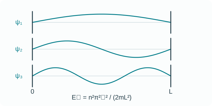
(a) Free particle. $V=0$ gives plane waves

$${\psi }_k(x,t)=\frac{1}{\sqrt{2\pi }}{e}^{i(kx-\omega t)},\omega =\frac{\hslash k^2}{2m}$$

Build wave packets by superposing $k$ values; packet center moves with group velocity $v_g=\hslash k/m$ and spreads over time.

(b) Infinite square well of width $L$ on $0<x<L$:

$${\varphi }_n(x)=\sqrt{\frac{2}{L}}\sin \left(\frac{n\pi x}{L}\right),E_n=\frac{{\hslash }^2{\pi }^2{n}^2}{2m{L}^2},n=1,2,\dots$$

Real eigenfunctions $\Rightarrow$ current $j=0$ in stationary states. Superpositions can carry current.

(c) Finite step and barriers. Impose continuity of $\varphi$ and ${\varphi }^{\prime }$ to get reflection $R$ and transmission $T$; probability flux conservation enforces $R+T=1$ for real potentials. For barriers, tunneling gives $T\sim e^{-2\kappa a}$ with $\kappa =\sqrt{2m(V_0-E)}/\hslash$ and width $a$.

7.2.7 Probability current in 1D scattering

For a stationary scattering state $\psi (x)=A_{\text{in}}{e}^{ikx}+A_{\text{re}}{e}^{-ikx}$ on the left and $\psi (x)=A_{\text{tr}}{e}^{i{k}^{\prime }x}$ on the right, the fluxes

$$j_{\text{in}}=\frac{\hslash k}{m}|A_{\text{in}}{|}^2,j_{\text{re}}=\frac{\hslash k}{m}|A_{\text{re}}{|}^2,j_{\text{tr}}=\frac{\hslash k^{\prime }}{m}|A_{\text{tr}}{|}^2$$

define reflection and transmission

$$R=\frac{j_{\text{re}}}{j_{\text{in}}},T=\frac{j_{\text{tr}}}{j_{\text{in}}}$$

For real $V$, $R+T=1$ follows from the continuity equation.

Detailed Explanation

Setup (incoming + reflected on the left, transmitted on the right):

For $x\to -\infty$:

$${\psi }_L(x)=A_{\text{in}}{e}^{ikx}+A_{\text{re}}{e}^{-ikx},k=\frac{\sqrt{2m(E-V_L)}}{\hslash }$$

For $x\to +\infty$:

$${\psi }_R(x)=A_{\text{tr}}{e}^{i{k}^{\prime }x},k^{\prime }=\frac{\sqrt{2m(E-V_R)}}{\hslash }$$

Here $V_L,V_R$ are constants, with $E>\max \{V_L,V_R\}$.

1) Continuity equation and probability flux

The time-dependent Schrödinger equation is

$$i\hslash \frac{\partial \psi }{\partial t}=-\frac{{\hslash }^2}{2m}\frac{{\partial }^2\psi }{\partial x^2}+V(x)\psi .$$

Its complex conjugate is

$$-i\hslash \frac{\partial {\psi }^{\ast }}{\partial t}=-\frac{{\hslash }^2}{2m}\frac{{\partial }^2{\psi }^{\ast }}{\partial x^2}+V(x){\psi }^{\ast }.$$

Multiplying the first by ${\psi }^{\ast }$ and the second by $\psi$, then subtracting, gives

$$i\hslash ({\psi }^{\ast }\frac{\partial \psi }{\partial t}+\psi \frac{\partial {\psi }^{\ast }}{\partial t})=-\frac{{\hslash }^2}{2m}[{\psi }^{\ast }\frac{{\partial }^2\psi }{\partial x^2}-\psi \frac{{\partial }^2{\psi }^{\ast }}{\partial x^2}]+\cancel{(V-V)|\psi {|}^2}.$$

The left-hand side becomes

$$i\hslash \frac{\partial }{\partial t}|\psi {|}^2,$$

and the right-hand side can be written as a total derivative:

$$-\frac{{\hslash }^2}{2m}\frac{\partial }{\partial x}[{\psi }^{\ast }\frac{\partial \psi }{\partial x}-(\frac{\partial {\psi }^{\ast }}{\partial x}\left)\psi \right].$$

Thus, for real $V(x)$,

$$\frac{\partial }{\partial t}|\psi {|}^2+\frac{\partial }{\partial x}j(x,t)=0,$$

with the probability flux

$$j(x,t)=\frac{\hslash }{2mi}[{\psi }^{\ast }\frac{\partial \psi }{\partial x}-(\frac{\partial {\psi }^{\ast }}{\partial x}\left)\psi \right].$$

For a stationary state $\psi (x,t)=\psi (x)e^{-iEt/\hslash }$,
${\partial }_t|\psi {|}^2=0$, so

$$\frac{d}{dx}j(x)=0\Rightarrow j(x)=\text{constant}.$$

2) Flux on the left side

On the left,

$${\psi }_L(x)=A_{\text{in}}{e}^{ikx}+A_{\text{re}}{e}^{-ikx}.$$

Derivative and conjugate:

$$\frac{d{\psi }_L}{dx}=ik{A}_{\text{in}}{e}^{ikx}-ik{A}_{\text{re}}{e}^{-ikx},{\psi }_L^{\ast }=A_{\text{in}}^{\ast }{e}^{-ikx}+A_{\text{re}}^{\ast }{e}^{ikx}.$$

Compute

$${\psi }_L^{\ast }\frac{d{\psi }_L}{dx}=(A_{\text{in}}^{\ast }{e}^{-ikx}+A_{\text{re}}^{\ast }{e}^{ikx})(ik{A}_{\text{in}}{e}^{ikx}-ik{A}_{\text{re}}{e}^{-ikx}).$$

Expansion gives

$$=ik|A_{\text{in}}{|}^2-ik|A_{\text{re}}{|}^2+ik(-A_{\text{in}}^{\ast }{A}_{\text{re}}{e}^{-2ikx}+A_{\text{re}}^{\ast }{A}_{\text{in}}{e}^{2ikx}).$$

Similarly,

$$\left(\frac{d{\psi }_L^{\ast }}{dx}\right){\psi }_L=(-ik{A}_{\text{in}}^{\ast }{e}^{-ikx}+ik{A}_{\text{re}}^{\ast }{e}^{ikx})(A_{\text{in}}{e}^{ikx}+A_{\text{re}}{e}^{-ikx}),$$

which expands to

$$=-ik|A_{\text{in}}{|}^2+ik|A_{\text{re}}{|}^2+ik(-A_{\text{in}}^{\ast }{A}_{\text{re}}{e}^{-2ikx}+A_{\text{re}}^{\ast }{A}_{\text{in}}{e}^{2ikx}).$$

Subtracting cancels the interference terms:

$${\psi }_L^{\ast }\frac{d{\psi }_L}{dx}-\left(\frac{d{\psi }_L^{\ast }}{dx}\right){\psi }_L=2ik(|A_{\text{in}}{|}^2-|A_{\text{re}}{|}^2).$$

Therefore

$$j_L=\frac{\hslash }{2mi}\cdot 2ik(|A_{\text{in}}{|}^2-|A_{\text{re}}{|}^2)=\frac{\hslash k}{m}(|A_{\text{in}}{|}^2-|A_{\text{re}}{|}^2).$$

Defining

$$j_{\text{in}}=\frac{\hslash k}{m}|A_{\text{in}}{|}^2,j_{\text{re}}=\frac{\hslash k}{m}|A_{\text{re}}{|}^2,$$

we find

$$j_L=j_{\text{in}}-j_{\text{re}}.$$

3) Flux on the right side

On the right,

$${\psi }_R(x)=A_{\text{tr}}{e}^{i{k}^{\prime }x}.$$

Derivative and conjugate:

$$\frac{d{\psi }_R}{dx}=i{k}^{\prime }{A}_{\text{tr}}{e}^{i{k}^{\prime }x},{\psi }_R^{\ast }=A_{\text{tr}}^{\ast }{e}^{-i{k}^{\prime }x}.$$

Thus,

$${\psi }_R^{\ast }\frac{d{\psi }_R}{dx}-\left(\frac{d{\psi }_R^{\ast }}{dx}\right){\psi }_R=2i{k}^{\prime }|A_{\text{tr}}{|}^2.$$

Hence

$$j_R=\frac{\hslash }{2mi}\cdot 2i{k}^{\prime }|A_{\text{tr}}{|}^2=\frac{\hslash k^{\prime }}{m}|A_{\text{tr}}{|}^2\equiv j_{\text{tr}}.$$

4) Conservation of flux $\Rightarrow R+T=1$

Stationarity and real $V(x)$ imply $j(x)$ is constant:

$$j_L=j_R.$$

Therefore,

$$j_{\text{in}}-j_{\text{re}}=j_{\text{tr}}\Rightarrow j_{\text{in}}=j_{\text{re}}+j_{\text{tr}}.$$

Define reflection and transmission:

$$R=\frac{j_{\text{re}}}{j_{\text{in}}},T=\frac{j_{\text{tr}}}{j_{\text{in}}}.$$

Finally,

$$1=\frac{j_{\text{re}}}{j_{\text{in}}}+\frac{j_{\text{tr}}}{j_{\text{in}}}\Rightarrow \boxed{R+T=1}.$$

Remark:
If $V(x)$ is complex (absorptive), the continuity equation gains a source term

$$\frac{\partial j}{\partial x}=\frac{2}{\hslash }\mathrm{Im}V(x)|\psi (x){|}^2,$$

so in general $R+T<1$.

7.2.8 Ehrenfest’s theorem (centers move classically)

Even in full quantum dynamics,

$$\frac{d}{dt}⟨\hat{x}⟩=\frac{⟨\hat{p}⟩}{m},\frac{d}{dt}⟨\hat{p}⟩=-⟨\frac{\partial V}{\partial x}⟩$$

When $\psi$ is narrow and $V$ is smooth, $⟨\partial V/\partial x⟩\approx \partial V(⟨x⟩)/\partial x$, so the packet centroid obeys Newton’s law while spread and interference track the departures.

7.2.9 Nodes, phases, and currents in bound states

For time-independent, real $V$, stationary bound eigenfunctions can be chosen real, so

$$\mathbf{j}=0$$

The quantum number $n$ counts nodes (zeros) of ${\varphi }_n$ in 1D wells; higher $n$ means more oscillations and higher energy. Relative phases only matter in superpositions, where interference redistributes probability and can create nonzero currents even in confining potentials.

7.2.10 Units and rescalings you will actually use

Set natural or atomic units to declutter:

• Natural: $\hslash =c=1$ for relativistic work
• Atomic (nonrelativistic electrons): $\hslash =m_e=e=4\pi {\epsilon }_0=1$, so energies in Hartrees and lengths in Bohr radii

Dimensionless rescaling often turns $\hat{H}$ into a minimal form with one control parameter, improving numerics and insight.

7.2.11 Worked mini-examples

(a) Normalization of a Gaussian packet

Take $\psi (x,0)=C{e}^{-(x-x_0{)}^2/(4{\sigma }^2)}{e}^{i{k}_{0}x}$. Enforce $\int |\psi {|}^{2}dx=1$ to get

$$C=\frac{1}{(2\pi {\sigma }^2{)}^{1/4}}$$

Time evolution preserves normalization.

(b) Expectation values in the well

For ${\varphi }_n$ in the infinite well, symmetry gives $⟨x⟩=L/2$ and

$$⟨x^2⟩=\frac{L^2}{3}-\frac{L^2}{2{\pi }^2{n}^2}$$

so the spatial spread increases with $n$ toward the classical uniform-distribution limit.

(c) Jump across a delta spike

For $V(x)=\lambda \delta (x)$, continuity $\varphi (0^{+})=\varphi (0^{-})$ and derivative jump

$${\varphi }^{\prime }(0^{+})-{\varphi }^{\prime }(0^{-})=\frac{2m\lambda }{{\hslash }^2}\varphi (0)$$

lead to one bound state at $E=-m{\lambda }^2/(2{\hslash }^2)$ for $\lambda <0$.

7.3 The Quantum Harmonic Oscillator: Algebra, Waves, and Coherent Motion

The harmonic oscillator is quantum’s Swiss Army knife. It models vibrations, phonons, molecular stretches, the EM field’s normal modes, even the “zero-point jitter” of everything. It is also where the math becomes elegant: one potential, two complementary solutions—differential (Hermite polynomials) and algebraic (ladder operators)—and a gallery of physical insights.

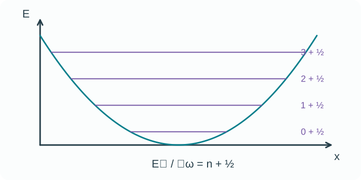
7.3.1 Setup and natural scales

Consider a 1D particle of mass $m$ with

$$V(x)=\frac{1}{2}m{\omega }^2{x}^2$$

Two natural scales declutter the algebra:

$$x_0\equiv \sqrt{\frac{\hslash }{m\omega }},p_0\equiv \sqrt{m\hslash \omega }$$

Introduce a dimensionless coordinate $\xi \equiv x/x_0$. We will hop between $x$ and $\xi$ as convenient.

7.3.2 Differential solution: Hermite world

The time-independent Schrödinger equation

$$-\frac{{\hslash }^2}{2m}\frac{d^2\varphi }{d{x}^2}+\frac{1}{2}m{\omega }^2{x}^2\varphi =E\varphi$$

becomes, in $\xi$,

$$\frac{d^2\varphi }{d{\xi }^2}+\left(2ϵ-{\xi }^2\right)\varphi =0,ϵ\equiv \frac{E}{\hslash \omega }$$

Normalizable solutions exist only when the series terminates, yielding Hermite polynomials $H_n(\xi )$ and the quantized spectrum

$$E_n=\hslash \omega \left(n+\frac{1}{2}\right),n=0,1,2,\dots$$

The normalized eigenfunctions are

$${\varphi }_n(x)=\frac{1}{{\pi }^{1/4}\sqrt{2^{n}n!x_0}}{H}_n\left(\frac{x}{x_0}\right)\exp \left(-\frac{x^2}{2x_0^2}\right)$$

Orthogonality and completeness follow from Hermite properties; nodes increase with $n$ and sit where $H_n$ changes sign.

7.3.3 Algebraic solution: ladder operators in 3 lines

Define

$$a\equiv \frac{1}{\sqrt{2}}\left(\frac{x}{x_0}+i\frac{p}{p_0}\right),a^{†}\equiv \frac{1}{\sqrt{2}}\left(\frac{x}{x_0}-i\frac{p}{p_0}\right)$$

These satisfy

$$[a,a^{†}]=1$$

The Hamiltonian becomes

$$H=\hslash \omega \left(a^{†}a+\frac{1}{2}\right)$$

with number operator $N\equiv a^{†}a$ and eigenstates $|n⟩$ such that

$$N|n⟩=n|n⟩,a|n⟩=\sqrt{n}|n-1⟩,a^{†}|n⟩=\sqrt{n+1}|n+1⟩$$

Algebra alone gives $E_n=\hslash \omega (n+\frac{1}{2})$, no differential equations needed.

7.3.4 Ground state and zero-point energy

The ground state obeys $a|0⟩=0$. In $x$-space this reads

$$\left(\frac{x}{x_0}+i\frac{p}{p_0}\right){\varphi }_0(x)=0$$

With $p\to -i\hslash {\partial }_x$ you recover the Gaussian

$${\varphi }_0(x)=\frac{1}{{\pi }^{1/4}\sqrt{x_0}}\exp \left(-\frac{x^2}{2x_0^2}\right)$$

Unavoidably, $E_0=\frac{1}{2}\hslash \omega$—the zero-point energy. No potential minimum is truly at rest in quantum mechanics.

7.3.5 Position and momentum matrix elements

Using $x=\frac{x_0}{\sqrt{2}}(a+a^{†})$ and $p=\frac{p_0}{\sqrt{2}}(a-a^{†})/i$,

$$⟨n^{\prime }|x|n⟩=\frac{x_0}{\sqrt{2}}\sqrt{n+1}{\delta }_{n^{\prime },n+1}+\frac{x_0}{\sqrt{2}}\sqrt{n}{\delta }_{n^{\prime },n-1}$$ $$⟨n^{\prime }|p|n⟩=\frac{i{p}_0}{\sqrt{2}}\sqrt{n+1}{\delta }_{n^{\prime },n+1}-\frac{i{p}_0}{\sqrt{2}}\sqrt{n}{\delta }_{n^{\prime },n-1}$$

Selection rule: only $\Delta n=\pm 1$ connect via $x$ or $p$, the oscillator’s dipole pattern.

7.3.6 Uncertainty and virial: clean checks

For the ground state,

$$\Delta x^2=\frac{x_0^2}{2}=\frac{\hslash }{2m\omega },\Delta p^2=\frac{p_0^2}{2}=\frac{m\hslash \omega }{2},\Delta x\Delta p=\frac{\hslash }{2}$$

A minimal-uncertainty state. For any stationary $|n⟩$ the quantum virial theorem gives

$$⟨T⟩=⟨V⟩=\frac{E_n}{2}$$

so half the energy sits in kinetic, half in potential—exactly as the classical time average.

7.3.7 Coherent states: quantum that cosplays classical

Define coherent states as eigenstates of $a$:

$$a|\alpha ⟩=\alpha |\alpha ⟩$$

Expand in number states to get

$$|\alpha ⟩=e^{-|\alpha {|}^2/2}\sum _{n=0}^{\infty }\frac{{\alpha }^n}{\sqrt{n!}}|n⟩$$

Time evolution is shape-preserving:

$$|\alpha (t)⟩=e^{-i\omega t/2}|\alpha e^{-i\omega t}⟩$$

Expectation values trace classical motion,

$$⟨x(t)⟩=x_0\sqrt{2}\Re \left[\alpha e^{-i\omega t}\right],⟨p(t)⟩=p_0\sqrt{2}\Im \left[\alpha e^{-i\omega t}\right]$$

while uncertainties remain constant and minimal, $\Delta x\Delta p=\hslash /2$. These states are the closest quantum analogs to phase-space points.

7.3.8 Forced oscillator and driven response

With a weak drive $H^{\prime }(t)=-F(t)x$, the Heisenberg equation for $a$ is linear, producing

$$\frac{da}{dt}=-i\omega a+\frac{i{x}_0}{\sqrt{2}\hslash }F(t)$$

A drive at frequency near $\omega$ displaces the coherent-state parameter $\alpha$ and yields resonant growth bounded by damping or finite interaction time. This is the quantum backbone of classical resonance and of light–matter coupling in cavity QED.

7.3.9 Hermite toolbox: recursions and nodes

Hermite polynomials satisfy

$$H_{n+1}(\xi )=2\xi H_n(\xi )-2n{H}_{n-1}(\xi )$$

and

$$\frac{d{H}_n}{d\xi }=2n{H}_{n-1}(\xi )$$

Zeros of $H_n$ are real and lie inside the classical turning points $\xi \approx \pm \sqrt{2n+1}$, foreshadowing the WKB picture where oscillatory regions live inside the turning points and exponential tails outside.

7.3.10 Creation of quanta: field-theory teaser

Because $H=\hslash \omega (N+\frac{1}{2})$, each $a^{†}$ raises the energy by one quantum $\hslash \omega$. Promoting $a,a^{†}$ to mode operators of a field turns the EM field into a set of independent oscillators, with $a^{†}$ creating a photon. Your oscillator algebra is literally second-quantization’s ABCs.

7.3.11 Worked mini-examples

(a) Expectation values in $|n⟩$.

Using $x\propto a+a^{†}$ and $N|n⟩=n|n⟩$,

$$⟨n|x|n⟩=0,⟨n|x^2|n⟩=\left(n+\frac{1}{2}\right)x_0^2$$

Similarly,

$$⟨n|p^2|n⟩=\left(n+\frac{1}{2}\right)p_0^2$$

Check that $⟨T⟩=⟨p^2⟩/(2m)=\frac{1}{2}{E}_n$.

(b) Transition matrix element $⟨n+1|x|n⟩$.

From $x=\frac{x_0}{\sqrt{2}}(a+a^{†})$,

$$⟨n+1|x|n⟩=\frac{x_0}{\sqrt{2}}\sqrt{n+1}$$

This controls dipole selection rules and line strengths for an oscillator-like transition.

(c) Overlap of coherent and number states.

The Poisson weights are

$$|⟨n|\alpha ⟩{|}^2=e^{-|\alpha {|}^2}\frac{|\alpha {|}^{2n}}{n!}$$

Mean quanta $\bar{n}=|\alpha {|}^2$ and variance $\Delta n^2=|\alpha {|}^2$.

7.3.12 Problem kit

• Derive the Hermite solution by power series, show termination, and recover $E_n$
• Starting from $a,a^{†}$, build $H$ and prove $E_n=\hslash \omega (n+\frac{1}{2})$ without solving a differential equation
• Compute $\Delta x$ and $\Delta p$ for ${\varphi }_0$ and verify the minimal-uncertainty product $\hslash /2$
• Show that $⟨x⟩$ for a coherent state follows $x_{\text{cl}}(t)$, while $|\psi (x,t){|}^2$ keeps a fixed Gaussian width
• Add a linear drive $F\cos \Omega t$ and solve for $a(t)$; identify the resonant response and phase lag
• Use $x=\frac{x_0}{\sqrt{2}}(a+a^{†})$ to prove that $⟨n^{\prime }|x|n⟩=0$ unless $n^{\prime }=n\pm 1$

7.4 Angular Momentum and Central Potentials

Before tackling hydrogen, we need the geometry engine of 3D quantum mechanics: angular momentum. Rotational symmetry gives conserved $\mathbf{L}$, spherical harmonics $Y_{\ell }^m$ carry the angles, and the radial Schrödinger equation sees an extra centrifugal barrier. This section builds the operator algebra, ladder machinery, spherical harmonics, and the central-potential separation that we will use on every spherically symmetric problem.

7.4.1 Angular momentum operators and algebra

Define orbital angular momentum

$$\mathbf{L}=\mathbf{r}\times \mathbf{p},L_i=-i\hslash {ϵ}_{ijk}{x}_j{\partial }_k$$

The commutators encode the rotation group

$$[L_i,L_j]=i\hslash {ϵ}_{ijk}{L}_k$$

The Casimir and components obey

$$L^2\equiv L_x^2+L_y^2+L_z^2,[L^2,L_i]=0$$

Because $[L^2,L_i]=0$, we can simultaneously diagonalize $L^2$ and one component, conventionally $L_z$.

7.4.2 Ladder operators and eigenvalue structure

Introduce

$$L_{\pm }\equiv L_x\pm i{L}_y$$

They satisfy

$$[L_z,L_{\pm }]=\pm \hslash L_{\pm },[L_{+},L_{-}]=2\hslash L_z$$

Let $|\ell m⟩$ be simultaneous eigenstates of $L^2$ and $L_z$

$$L^2|\ell m⟩={\hslash }^2\ell (\ell +1)|\ell m⟩,L_z|\ell m⟩=\hslash m|\ell m⟩$$

Ladders step $m$ within a fixed $\ell$

$$L_{\pm }|\ell m⟩=\hslash \sqrt{\ell (\ell +1)-m(m\pm 1)}|\ell ,m\pm 1⟩$$

Allowable quantum numbers are

$$\ell =0,1,2,\dots ,m=-\ell ,-\ell +1,\dots ,\ell$$

giving a $(2\ell +1)$-fold degeneracy for each $\ell$.

7.4.3 Spherical harmonics: the angular wavefunctions

In position representation the simultaneous eigenfunctions are the spherical harmonics $Y_{\ell }^m(\theta ,\varphi )$, obeying

$$L^2{Y}_{\ell }^m={\hslash }^2\ell (\ell +1)Y_{\ell }^m,L_z{Y}_{\ell }^m=\hslash m{Y}_{\ell }^m$$

with orthonormality and completeness on the unit sphere

$${\int }_0^{2\pi }{\int }_0^{\pi }{Y}_{\ell }^m(\theta ,\varphi {)}^{\ast }{Y}_{{\ell }^{\prime }}^{m^{\prime }}(\theta ,\varphi )\sin \theta d\theta d\varphi ={\delta }_{\ell {\ell }^{\prime }}{\delta }_{m{m}^{\prime }}$$ $$\sum _{\ell =0}^{\infty }\sum _{m=-\ell }^{\ell }{Y}_{\ell }^m(\Omega )Y_{\ell }^m({\Omega }^{\prime }{)}^{\ast }=\delta (\cos \theta -\cos {\theta }^{\prime })\delta (\varphi -{\varphi }^{\prime })$$

Parity is simple

$$Y_{\ell }^m(\pi -\theta ,\varphi +\pi )=(-1{)}^{\ell }{Y}_{\ell }^m(\theta ,\varphi )$$

Explicitly, with associated Legendre functions $P_{\ell }^m$,

$$Y_{\ell }^m(\theta ,\varphi )=N_{\ell m}{P}_{\ell }^m(\cos \theta )e^{im\varphi }$$

where $N_{\ell m}$ is the standard normalization constant.

7.4.4 Laplacian in spherical coordinates and separation of variables

The 3D Laplacian is

$${\nabla }^2=\frac{1}{r^2}\frac{\partial }{\partial r}\left(r^2\frac{\partial }{\partial r}\right)-\frac{L^2}{{\hslash }^2{r}^2}$$

For a central potential $V(r)$ the time-independent Schrödinger equation

$$\left[-\frac{{\hslash }^2}{2m}{\nabla }^2+V(r)\right]\psi (\mathbf{r})=E\psi (\mathbf{r})$$

separates with the ansatz $\psi (r,\theta ,\varphi )=R_{n\ell }(r)Y_{\ell }^m(\theta ,\varphi )$. The angular part yields the spherical harmonics above; the radial part obeys

$$-\frac{{\hslash }^2}{2m}\left[\frac{1}{r^2}\frac{d}{dr}\left(r^2\frac{dR}{dr}\right)-\frac{\ell (\ell +1)}{r^2}R\right]+V(r)R=ER$$

It is cleaner to remove the first derivative by $u(r)\equiv rR(r)$, giving the radial Schrödinger equation

$$-\frac{{\hslash }^2}{2m}\frac{d^{2}u}{d{r}^2}+\left[V(r)+\frac{{\hslash }^2\ell (\ell +1)}{2m{r}^2}\right]u=Eu$$

The bracketed term is the effective potential

$$V_{\text{eff}}(r)=V(r)+\frac{{\hslash }^2\ell (\ell +1)}{2m{r}^2}$$

with a quantum centrifugal barrier $\propto 1/r^2$.

7.4.5 Radial normalization and boundary conditions

Assuming angular functions are normalized, the full normalization reduces to

$${\int }_0^{\infty }|u(r){|}^{2}dr=1$$

Physical solutions satisfy

• Regularity at the origin: $u(r)\sim r^{\ell +1}$ as $r\to 0$ for finite $V(0)$
• Normalizability for bound states: $u(r)\to 0$ as $r\to \infty$
• Appropriate scattering asymptotics for $E>0$

These conditions quantize $E$ for confining $V(r)$.

7.4.6 Rotational symmetry, Noether, and degeneracy

If $V(r)$ is central, the Hamiltonian commutes with all rotations $U(R)=\exp \left(-\frac{i}{\hslash }\mathbf{\theta }\cdot \mathbf{L}\right)$. Noether’s theorem in the quantum language says

$$[H,\mathbf{L}]=0$$

Hence $\ell$ and $m$ label eigenstates. Energies depend on $n$ and $\ell$ in general, but are $m$-degenerate by $(2\ell +1)$ because rotating a solution merely mixes $m$ values inside the same $\ell$ multiplet.

Special symmetries can enlarge degeneracy. For hydrogen, a hidden Runge–Lenz symmetry makes $E$ depend on $n$ only; for the isotropic 3D oscillator, $E$ depends on $N=2n_r+\ell$.

7.4.7 Angular momentum as the generator of rotations

Infinitesimal rotations act as

$$\delta \psi (\mathbf{r})=-\frac{i}{\hslash }\delta \mathbf{\theta }\cdot \mathbf{L}\psi (\mathbf{r})$$

For a finite rotation $R$, the transformed state is $U(R)\psi$, with coordinates rotating oppositely. On the sphere, the $Y_{\ell }^m$ furnish irreducible representations of $SO(3)$; under $R$, components mix within fixed $\ell$ via Wigner $D$-matrices $D_{m^{\prime }m}^{(\ell )}(R)$.

7.4.8 Orbital vs spin, and addition (teaser)

Electrons carry orbital $\mathbf{L}$ and spin $\mathbf{S}$ angular momenta. The total

$$\mathbf{J}=\mathbf{L}+\mathbf{S}$$

obeys the same algebra as any angular momentum. When two angular momenta couple, the allowed totals $j$ follow triangle rules and states expand with Clebsch–Gordan coefficients. We will use these tools for fine structure, selection rules, and multi-particle systems later in the chapter.

7.4.9 Worked mini-examples

(a) Small-$r$ behavior of $u(r)$.
For finite $V(0)$, the dominant terms in the radial equation near $r=0$ are

$$-\frac{{\hslash }^2}{2m}{u}^{\prime \prime }(r)+\frac{{\hslash }^2\ell (\ell +1)}{2m{r}^2}u(r)\approx 0$$

Try $u\sim r^s$ to get $s(s-1)=\ell (\ell +1)$, giving $s=\ell +1$ (regular) and $s=-\ell$ (singular). Keep $u\sim r^{\ell +1}$.

(b) Expectation of $L^2$ in a separable state.
For $\psi =R(r)Y_{\ell }^m(\theta ,\varphi )$,

$$⟨L^2⟩={\hslash }^2\ell (\ell +1)$$

independent of $R(r)$ because angles carry all the $L$ structure.

(c) Degeneracy count at fixed $\ell$.
Show that the set $\{Y_{\ell }^m{\}}_{m=-\ell }^{\ell }$ spans a $(2\ell +1)$-dimensional irrep by applying $L_{\pm }$ repeatedly to $Y_{\ell }^{\ell }$ and $Y_{\ell }^{-\ell }$.

(d) Effective potential sketch.
For $V(r)=-k/r$ (Coulomb), plot $V_{\text{eff}}(r)=-k/r+{\hslash }^2\ell (\ell +1)/(2m{r}^2)$ to visualize classical-like turning points and bound-state regions for various $\ell$.

7.4.10 Minimal problem kit

• Starting from ${\nabla }^2$ in spherical coordinates, derive the radial equation for $u(r)$ and identify $V_{\text{eff}}(r)$
• Prove the ladder action of $L_{\pm }$ on $|\ell m⟩$ and normalize the coefficients by demanding $⟨\ell m|\ell m⟩=1$
• Verify orthonormality of $Y_{\ell }^m$ by integrating two explicit low-$\ell$ examples over the sphere
• For a central square well $V(r)=-V_0$ for $r<R$ and $0$ otherwise, write the bound-state matching conditions for $u(r)$ at $r=R$ and discuss $\ell$-dependence of the spectrum
• Show that $[H,\mathbf{L}]=0$ for any $V(r)$ and use it to argue $(2\ell +1)$ degeneracy in $m$

7.5 The Hydrogen Atom: Solving the Coulomb Problem

This is the first full 3D victory lap of quantum mechanics. With rotational symmetry from §7.4 and the Coulomb potential, we separate variables, solve the radial equation, get exact energy levels

$$E_n=-\frac{\mu e^4}{2(4\pi {\epsilon }_0{)}^2{\hslash }^2}\frac{Z^2}{n^2}=-\frac{\mu c^2{\alpha }^2}{2}\frac{Z^2}{n^2}$$

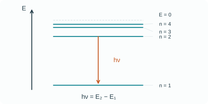
and explicit wavefunctions labeled by $(n,\ell ,m)$. Hydrogen wins because the math secretly has extra symmetry; the degeneracy is $n^2$ per $n$ (ignoring spin).

7.5.1 Setup and separation

Take a nucleus of charge $+Ze$ and an electron of charge $-e$. Use the reduced mass

$$\mu \equiv \frac{m_e{m}_N}{m_e+m_N}$$

and the Coulomb constant

$$k\equiv \frac{Z{e}^2}{4\pi {\epsilon }_0}$$

The time-independent Schrödinger equation with a central potential $V(r)=-k/r$ separates as $\psi (r,\theta ,\varphi )=R_{n\ell }(r)Y_{\ell }^m(\theta ,\varphi )$. The radial function $u(r)\equiv rR(r)$ obeys

$$-\frac{{\hslash }^2}{2\mu }\frac{d^{2}u}{d{r}^2}+\left[\frac{{\hslash }^2\ell (\ell +1)}{2\mu r^2}-\frac{k}{r}\right]u=Eu$$

Bound states have $E<0$.

7.5.2 Non-dimensionalization and solution shape

Define

$$\kappa \equiv \frac{\sqrt{-2\mu E}}{\hslash },\rho \equiv 2\kappa r$$

Look for solutions of the form

$$u(\rho )={\rho }^{\ell +1}{e}^{-\rho /2}v(\rho )$$

Regularity and normalizability force $v(\rho )$ to be a polynomial, specifically an associated Laguerre

$$v(\rho )\propto L_{n-\ell -1}^{2\ell +1}(\rho )$$

and quantization pops out as

$$\kappa =\frac{\mu k}{{\hslash }^2}\frac{1}{n},n=1,2,3,\dots$$

which yields the spectrum quoted above.

7.5.3 Bohr radius, length scale, and quantum numbers

Introduce the reduced-mass Bohr radius

$$a_{\mu }\equiv \frac{4\pi {\epsilon }_0{\hslash }^2}{\mu e^2}$$

and the hydrogenic length

$$a\equiv \frac{a_{\mu }}{Z}$$

Quantum numbers:

• Principal $n=1,2,\dots$
• Orbital $\ell =0,1,\dots ,n-1$
• Magnetic $m=-\ell ,-\ell +1,\dots ,\ell$

For each $n$, the total degeneracy is

$$\sum _{\ell =0}^{n-1}(2\ell +1)=n^2$$

Doubling by electron spin gives $2n^2$.

7.5.4 Radial wavefunctions and normalization

With $a=a_{\mu }/Z$, the normalized hydrogenic radial functions are

$$R_{n\ell }(r)=\frac{2}{n^2{a}^{3/2}}\sqrt{\frac{(n-\ell -1)!}{(n+\ell )!}}\exp \left(-\frac{r}{na}\right){\left(\frac{2r}{na}\right)}^{\ell }{L}_{n-\ell -1}^{2\ell +1}\left(\frac{2r}{na}\right)$$

so that

$${\int }_0^{\infty }|R_{n\ell }(r){|}^2{r}^{2}dr=1$$

Sanity checks:

• $1s$ $(n=1,\ell =0)$ gives $R_{10}(r)=2a^{-3/2}{e}^{-r/a}$
• $2p$ $(n=2,\ell =1)$ gives $R_{21}(r)\propto r{e}^{-r/(2a)}$

7.5.5 Probability, nodes, and orbital shapes

The radial probability density is

$$P_{n\ell }(r)=|R_{n\ell }(r){|}^2{r}^2$$

Node counting:

• Angular: $\ell$ nodal planes/surfaces from $Y_{\ell }^m$
• Radial: $n-\ell -1$ nodes from $R_{n\ell }$

Peaks move outward with $n$; for $1s$, $P$ peaks at $r=a$.

7.5.6 Useful expectation values

In terms of $a=a_{\mu }/Z$,

$$⟨\frac{1}{r}{⟩}_{n\ell }=\frac{1}{n^{2}a}$$ $$⟨r{⟩}_{n\ell }=\frac{a}{2}\left[3n^2-\ell (\ell +1)\right]$$ $$⟨r^2{⟩}_{n\ell }=a^2\frac{n^2}{2}\left[5n^2+1-3\ell (\ell +1)\right]$$

These nail orders of magnitude for atom size and screening estimates.

7.5.7 Dipole selection rules and lines

For electric-dipole radiation with $\hat{\mathbf{d}}=-e\mathbf{r}$,

$$\Delta \ell =\pm 1,\Delta m=0,\pm 1$$

Line strengths follow from matrix elements

$$⟨n^{\prime }{\ell }^{\prime }{m}^{\prime }|\mathbf{r}|n\ell m⟩$$

which factor into angular pieces (Clebsch–Gordan algebra) and radial integrals built from the $R_{n\ell }(r)$. This reproduces the Balmer/Lyman series patterns and polarization rules.

7.5.8 Runge–Lenz symmetry and $n$-only energy

The Coulomb problem has a conserved Runge–Lenz vector (quantum-symmetrized)

$$\mathbf{A}=\frac{1}{2\mu }(\mathbf{p}\times \mathbf{L}-\mathbf{L}\times \mathbf{p})-k\hat{\mathbf{r}}$$

Together, $\mathbf{L}$ and $\mathbf{A}$ generate an $SO(4)$ symmetry for bound states, explaining why $E_n$ depends on $n$ only, not on $\ell$ or $m$. Break that symmetry (e.g., by fields or relativity) and the degeneracy splits.

7.5.9 Real-world splittings: what lifts the degeneracy

Hydrogen is not perfectly degenerate once we add small effects:

• Reduced mass. Already included by $\mu$; shifts $R_{\text{H}}$ slightly and creates isotope shifts
• Fine structure. Relativistic kinetic correction, spin–orbit coupling, and Darwin term split levels by order ${\alpha }^2$ of the Rydberg; handled by perturbation theory in §7.6
• Lamb shift. QED vacuum fluctuations separate $2S$ and $2P$ levels (famously nonzero)
• Hyperfine. Proton–electron spin coupling yields the 21-cm line; scales with magnetic moments and wavefunction at the origin

Each effect has a clean perturbative footprint, making hydrogen a precision playground.

7.5.10 Worked mini-examples

(a) Most probable radius for $1s$.

Maximize $P_{10}(r)=4r^2{a}^{-3}{e}^{-2r/a}$. The derivative zero gives $r=a$.

(b) Rydberg constant from the spectrum.

The photon wavenumber between $n\to n^{\prime }$ is

$$\tilde{\nu }=\frac{E_n-E_{n^{\prime }}}{hc}=R_{\infty }\frac{\mu }{m_e}{Z}^2\left(\frac{1}{n^{\prime 2}}-\frac{1}{n^2}\right)$$

with

$$R_{\infty }=\frac{{\alpha }^2{m}_{e}c}{2h}$$

(c) Radial integral for $2p\to 1s$.

The dipole matrix element reduces to

$$⟨1s||r||2p⟩={\int }_0^{\infty }{R}_{10}(r)r{R}_{21}(r)r^{2}dr$$

Plugging the explicit $R$’s gives a nonzero value, consistent with $\Delta \ell =1$.

(d) Expectation of $1/r$ from Virial.

For $V\propto 1/r$, the virial theorem yields $⟨T⟩=-E$ and $⟨V⟩=2E$, hence

$$⟨\frac{1}{r}⟩=\frac{-2E}{k}=\frac{1}{n^{2}a}$$

matching the formula above.

7.5.11 Minimal problem kit

• Starting from the radial equation, perform the $\rho =2\kappa r$ substitution and show that termination of the Laguerre series gives $n=\ell +1+n_r$ and $E_n\propto -1/n^2$
• Derive and normalize $R_{10}(r)$ and $R_{21}(r)$ explicitly
• Prove the degeneracy count ${\sum }_{\ell =0}^{n-1}(2\ell +1)=n^2$ and extend to $2n^2$ with spin
• Compute $⟨r{⟩}_{n\ell }$ using orthogonality of associated Laguerres
• Evaluate the angular selection rules for dipole transitions via Wigner–Eckart or Clebsch–Gordan coefficients
• Estimate the fine-structure splitting for $n=2$ levels using leading relativistic and spin–orbit terms as a teaser for §7.6

7.6 Time-Independent Perturbation Theory: Nondegenerate, Degenerate, and First Applications

Real systems are rarely exactly solvable, but many are almost solvable. Perturbation theory is the art of starting from a Hamiltonian you can diagonalize, then adding a small extra term and tracking how energies and states shift. It powers fine structure in hydrogen, Zeeman/Stark effects, chemical shifts, and basically every “small correction” you care about.

7.6.1 Setup and the expansion game

Let

$$H(\lambda )=H_0+\lambda H^{\prime }$$

where $H_0$ is solvable with eigenpairs $\{E_n^{(0)},|n^{(0)}⟩\}$ and $H^{\prime }$ is the perturbation. Seek series

$$E_n=E_n^{(0)}+\lambda E_n^{(1)}+{\lambda }^2{E}_n^{(2)}+\cdots$$ $$|n⟩=|n^{(0)}⟩+\lambda |n^{(1)}⟩+{\lambda }^2|n^{(2)}⟩+\cdots$$

Adopt intermediate normalization $⟨n^{(0)}|n⟩=1$, which implies $⟨n^{(0)}|n^{(k)}⟩=0$ for $k\ge 1$ and keeps formulas tidy.

7.6.2 Nondegenerate perturbation theory

Assume $E_n^{(0)}$ is nondegenerate.

First-order energy

$$E_n^{(1)}=⟨n^{(0)}|H^{\prime }|n^{(0)}⟩$$

First-order state

$$|n^{(1)}⟩=\sum _{m\ne n}\frac{|m^{(0)}⟩⟨m^{(0)}|H^{\prime }|n^{(0)}⟩}{E_n^{(0)}-E_m^{(0)}}$$

Second-order energy

$$E_n^{(2)}=\sum _{m\ne n}\frac{|⟨m^{(0)}|H^{\prime }|n^{(0)}⟩{|}^2}{E_n^{(0)}-E_m^{(0)}}$$

Sign check: if $H^{\prime }$ mixes $n$ with higher states, denominators are negative so $E_n$ typically drops.

Selection rules: many matrix elements vanish by symmetry (parity, angular momentum), so first-order shifts can be zero and second-order becomes the leading term.

7.6.3 Hellmann–Feynman and quick derivatives

If $H(\lambda )$ depends smoothly on a parameter $\lambda$ and $|n(\lambda )⟩$ is an exact eigenstate,

$$\frac{d{E}_n}{d\lambda }=⟨n(\lambda )\left|\frac{\partial H}{\partial \lambda }\right|n(\lambda )⟩$$

This avoids differentiating messy wavefunctions: compute the expectation of the explicit derivative of $H$. Great for forces in molecules and for tracking how $E$ slides with external fields.

7.6.4 Degenerate perturbation theory

If several $H_0$ eigenstates share the same $E^{(0)}$, the nondegenerate perturbation formulas have zero denominators. Fix by diagonalizing $H^{\prime }$ within the degenerate subspace.

Let $\{|{\varphi }_a⟩{\}}_{a=1}^g$ be an orthonormal basis of a $g$-fold degenerate eigenspace of $H_0$. Build the secular matrix

$$W_{ab}\equiv ⟨{\varphi }_a|H^{\prime }|{\varphi }_b⟩$$

Diagonalize $W$ to get eigenvalues $\{{\lambda }_{\alpha }\}$ and eigenvectors $\{{\mathbf{c}}^{(\alpha )}\}$. Then

$$E_{\alpha }^{(1)}={\lambda }_{\alpha }$$ $$|{\psi }_{\alpha }^{(0)}⟩=\sum _{a=1}^g{c}_a^{(\alpha )}|{\varphi }_a⟩$$

These optimized zeroth-order states already include the dominant mixing; higher orders then proceed as in the nondegenerate case using $|{\psi }_{\alpha }^{(0)}⟩$.

Rule of thumb: choose a basis adapted to the symmetries of $H^{\prime }$. You will often find that $W$ block-diagonalizes (e.g., fixed $m$ or fixed parity), making life easy.

7.6.5 First applications: hydrogen fine structure (order ${\alpha }^4$)

For $Z{e}^2/4\pi {\epsilon }_{0}r$ with $Z=1$, three relativistic corrections dress $H_0$:

1. Relativistic kinetic energy

$$H_{\mathrm{rel}}=-\frac{p^4}{8m_e^3{c}^2}$$

2. Spin–orbit coupling with Thomas factor

$$H_{\mathrm{SO}}=\frac{1}{2m_e^2{c}^2}\frac{1}{r}\frac{dV}{dr}\mathbf{L}\cdot \mathbf{S}$$

For Coulomb $V(r)=-e^2/4\pi {\epsilon }_{0}r$, this is $\propto +\mathbf{L}\cdot \mathbf{S}/r^3$

3. Darwin term (contact term from Zitterbewegung, nonzero only for $\ell =0$)

$$H_{\mathrm{D}}=\frac{{\hslash }^2}{8m_e^2{c}^2}{\nabla }^{2}V(r)$$

Combine expectation values using hydrogen eigenstates and angular momentum algebra. The sum depends on $n$ and the total $j=\ell \pm \frac{1}{2}$ but not on $m$, giving the textbook fine-structure shift

$$\Delta E_{n,j}^{(\mathrm{fs})}=-\frac{\mu c^2(Z\alpha {)}^4}{2n^3}\left(\frac{1}{j+\frac{1}{2}}-\frac{3}{4n}\right)$$

Here $\mu$ is the reduced mass and $\alpha \equiv e^2/4\pi {\epsilon }_0\hslash c$. Fine structure splits the spin-inclusive $2n^2$ degeneracy according to $j$. Each allowed angular-momentum multiplet retains $2j+1$ magnetic states labeled by $m$; states with the same principal and total angular-momentum quantum numbers but different orbital angular momentum remain degenerate at this order.

7.6.6 Zeeman effect: weak magnetic fields

Add a uniform magnetic field $\mathbf{B}=B\hat{\mathbf{z}}$. The leading coupling is

$$H_{\mathrm{Z}}^{\prime }=\frac{{\mu }_B}{\hslash }(L_z+g_s{S}_z)B$$

with $g_s\approx 2$ and ${\mu }_B=e\hslash /2m_e$. In LS coupling, levels are labeled by $|n\ell sj{m}_j⟩$ and the shift is packaged as

$$\Delta E_{\mathrm{Z}}={\mu }_B{g}_J{m}_{J}B$$

where the Landé factor

$$g_J=1+\frac{j(j+1)+s(s+1)-\ell (\ell +1)}{2j(j+1)}$$

For $s=\frac{1}{2}$, this reproduces the familiar “anomalous” Zeeman patterns. The selection rule for dipole transitions remains $\Delta m_J=0,\pm 1$; polarizations track $\pi$ and ${\sigma }^{\pm }$ components.

Strong-field (Paschen–Back) note: when ${\mu }_{B}B$ beats spin–orbit, $L$ and $S$ uncouple and you diagonalize $L_z$ and $S_z$ instead of $J^2$, but that is beyond first-order weak-field PT.

7.6.7 Stark effect: electric fields and parity trouble

For a static electric field $\mathbf{E}=E\hat{\mathbf{z}}$,

$$H_{\mathrm{S}}^{\prime }=eEz$$

Parity makes first-order shifts vanish in nondegenerate levels with definite parity (e.g., hydrogen $1s$). Thus the leading shift is second order:

$$\Delta E^{(2)}=\sum _{m\ne n}\frac{|⟨m^{(0)}|eEz|n^{(0)}⟩{|}^2}{E_n^{(0)}-E_m^{(0)}}$$

For hydrogen $1s$ this yields a quadratic Stark shift

$$\Delta E_{1s}=-\frac{1}{2}{\alpha }_{1s}{E}^2,{\alpha }_{1s}=\frac{9}{2}(4\pi {\epsilon }_0)a_0^3$$

where $\alpha$ is the polarizability and $a_0$ the Bohr radius.

Linear Stark in degenerate manifolds. When $H_0$ has degeneracy of opposite parities (hydrogen $n\ge 2$), do degenerate PT in the $n$ manifold using parabolic states. First-order shifts appear:

$$\Delta E_{n,k,m}=\frac{3}{2}ne{a}_{0}Ek$$

with $k=n_1-n_2$ the parabolic quantum number satisfying $n_1+n_2+|m|+1=n$. For $n=2$, $k=\pm 1$ at $m=0$ split linearly, while $|m|=1$ states stay unshifted at first order.

7.6.8 Practical workflow and symmetry hacks

• Exploit good quantum numbers. Work in a basis that diagonalizes all operators commuting with both $H_0$ and $H^{\prime }$
• Use Wigner–Eckart to drop angles. For dipole-type perturbations $r_q$, factor angular parts into Clebsch–Gordan coefficients and a reduced matrix element so you only carry one radial integral
• Mind selection rules. If first order vanishes by symmetry, skip straight to second order (saves algebra and surprises)
• Estimate sizes early. Compare typical matrix elements of $H^{\prime }$ to level spacings of $H_0$. If the ratio is not $\ll 1$, perturbation theory will not slay this dragon

7.6.9 Worked mini-examples

(a) Quadratic Stark for hydrogen ground state

Use the complete set of $np$ bound states together with the continuum p-wave states to show

$$\Delta E_{1s}^{(2)}=-\frac{1}{2}{\alpha }_{1s}{E}^2,{\alpha }_{1s}=\frac{9}{2}(4\pi {\epsilon }_0)a_0^3$$

Sketch: only $\ell =1$ intermediate states contribute because $z\propto Y_1^0$ changes $\ell$ by $\pm 1$. Evaluate the radial sum or use known hydrogenic polarizability.

(b) Zeeman splitting of a $2P_{3/2}$ level

With $j=\frac{3}{2}$, $g_J=\frac{4}{3}$. Allowed $m_J=\{-\frac{3}{2},-\frac{1}{2},\frac{1}{2},\frac{3}{2}\}$ produce four equally spaced lines with separation ${\mu }_B{g}_{J}B$.

(c) Fine-structure order of magnitude

For $n=2$, the scale is

$$|\Delta E^{(\mathrm{fs})}|\sim \mu c^2{\alpha }^4/16$$

which for hydrogen lands in the $10^{-4}\text{eV}$ range, i.e., tens of GHz—microwave domain.

(d) Two-level avoided crossing via second order

For a pair $\{|1⟩,|2⟩\}$ with $E_2^{(0)}-E_1^{(0)}=\Delta$ and off-diagonal $⟨1|H^{\prime }|2⟩=V$, diagonalize

$$\left(\begin{array}{cc}{E}_1^{(0)}& V\\ V& E_2^{(0)}\end{array}\right)$$

to get exact $E_{\pm }=\frac{1}{2}(E_1^{(0)}+E_2^{(0)})\pm \frac{1}{2}\sqrt{{\Delta }^2+4V^2}$. For $|V|\ll |\Delta |$, recover second-order shifts $\pm V^2/\Delta$. This is the algebraic skeleton behind many “near-degenerate” perturbations.

7.6.10 Common pitfalls and how not to trip

• Forgetting to orthogonalize in degenerate spaces. Always diagonalize $H^{\prime }$ first; otherwise denominators lie to you
• Using unperturbed labels after mixing. Once you diagonalize $W$, the “good” zeroth-order states are the $W$ eigenvectors, not the original basis
• Boundary terms in Hellmann–Feynman. HF needs exact eigenstates; variational or truncated bases require adding Pulay-type corrections when the basis depends on $\lambda$
• Order counting. If first order vanishes, second order can be dominant but still “small.” Check scales before trusting the series

7.6.11 Minimal problem kit

• Derive $E_n^{(1)}$, $|n^{(1)}⟩$, and $E_n^{(2)}$ from the series ansatz with intermediate normalization
• For a 3-fold degenerate level $\{|{\varphi }_1⟩,|{\varphi }_2⟩,|{\varphi }_3⟩\}$ and perturbation $H^{\prime }$, build $W$, solve the secular equation $\det (W-\lambda I)=0$, and construct the mixed eigenkets
• Compute the Landé $g_J$ formula from $H_{\mathrm{Z}}^{\prime }$ using vector coupling and verify special cases $S$ ($\ell =0$) and $L$-only ($s=0$) limits
• Evaluate the quadratic Stark shift for $1s$ by explicit summation over $np$ bound states and integration over continuum p-wave states, or by an equivalent complete-resolvent method.
• Starting from $H_{\mathrm{rel}},H_{\mathrm{SO}},H_{\mathrm{D}}$, show that the combined fine-structure correction depends only on $n$ and $j$ and reproduce $\Delta E_{n,j}^{(\mathrm{fs})}$ above